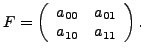
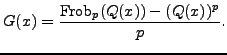
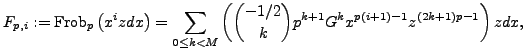
We focus on the computation of this matrix. Details omitted here can be found in the aforementioned papers.
Let
![]() denote the affine curve over
denote the affine curve over
![]() cut out
by the equation
cut out
by the equation
![]() . Consider
. Consider
![]() zeros of
zeros of ![]() , and let
, and let
denote the coordinate ring of
gives us an automorphism of the curves
The
![]() -vector space
-vector space
![]() is spanned by the classes of
differentials
is spanned by the classes of
differentials
However, the underlying coordinate ring
The de Rham complex of
![]() is given by
is given by
 |
||
 |
 |
|
 |
We denote the cohomology groups of this complex by
![]() , and as before, they are
, and as before, they are
![]() -vector
spaces split into eigenspaces by the hyperelliptic involution.
Perhaps more important is that passing from
-vector
spaces split into eigenspaces by the hyperelliptic involution.
Perhaps more important is that passing from ![]() to
to
![]() does not change the presentation of cohomology, and thus we work
with
does not change the presentation of cohomology, and thus we work
with
![]() and its basis
and its basis ![]() and
and ![]() .
.
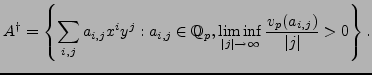
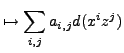
We compute the action of Frobenius on
![]() by computing its action on the basis elements. Begin by letting
by computing its action on the basis elements. Begin by letting
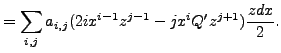
We have that
as an element of
As the two differentials ![]() and
and ![]() span
span
![]() , we must now be able to write an
arbitrary element in
, we must now be able to write an
arbitrary element in
![]() (where
(where
![]() as a linear
combination of
as a linear
combination of ![]() ,
, ![]() , and
, and ![]() . With this in
mind, we employ a reduction algorithm. For the purposes of this
reduction, the following definition is helpful:
. With this in
mind, we employ a reduction algorithm. For the purposes of this
reduction, the following definition is helpful:
is
Here we outline the reduction algorithm. Begin by computing a list
of differentials ![]() , where
, where
![]() and
and
![]() . Group the terms in
. Group the terms in
![]() as
as
![]() , where
, where
![]() have degree less than
or equal to 3.
have degree less than
or equal to 3.
If ![]() has a term
has a term
![]() with
with ![]() , consider the
term
, consider the
term
![]() where
where ![]() is maximal. Take the unique
linear combination of the
is maximal. Take the unique
linear combination of the
![]() such that when this
linear combination is subtracted off of
such that when this
linear combination is subtracted off of ![]() , the resulting
``
, the resulting
``![]() '' no longer has terms of the form
'' no longer has terms of the form
![]() .
Repeat this process until
.
Repeat this process until ![]() (or, in more precise terms,
the resulting ``
(or, in more precise terms,
the resulting ``![]() '' at each step minus linear combinations
of differentials) has no terms
'' at each step minus linear combinations
of differentials) has no terms
![]() with
with ![]() .
.
If ![]() has terms with
has terms with ![]() , let
, let
![]() be the
term with the highest monomial of
be the
term with the highest monomial of ![]() . Let
. Let
![]() be
the term such that
be
the term such that ![]() has highest term
has highest term
![]() and
subtract off the appropriate multiple of
and
subtract off the appropriate multiple of ![]() such that the
resulting
such that the
resulting ![]() no longer has terms of the form
no longer has terms of the form
![]() with
with ![]() . Repeat this process until the resulting
. Repeat this process until the resulting ![]() is of the form
is of the form
![]() .
.
Finally, we can read off the entries of the matrix ![]() of absolute
Frobenius:
of absolute
Frobenius: