Modular Forms of Level 1
In this chapter we study in detail the structure of level  modular
forms, i.e., modular forms on
modular
forms, i.e., modular forms on  We assume some complex analysis (e.g., the residue theorem),
linear algebra, and that the reader has
read Chapter Modular Forms.
We assume some complex analysis (e.g., the residue theorem),
linear algebra, and that the reader has
read Chapter Modular Forms.
Examples of Modular Forms of Level 1
In this section we will finally see some examples of modular forms of
level ! We first introduce the Eisenstein series and
then define  , which is a cusp form of weight
  . In
Section Structure Theorem for Level 1 Modular Forms we prove the structure theorem,
which says that all modular forms of level are polynomials
in Eisenstein series.
. In
Section Structure Theorem for Level 1 Modular Forms we prove the structure theorem,
which says that all modular forms of level are polynomials
in Eisenstein series.
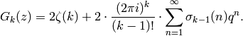
For an even integer  , the
nonnormalized weight
, the
nonnormalized weight  Eisenstein series is the
function on the extended upper half plane
Eisenstein series is the
function on the extended upper half plane
 given by
(1)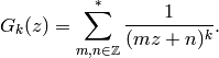
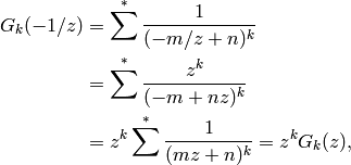
The star on top of the sum symbol means that
for each  the sum is over all
  such that
 .
.
Proposition 2.1
The function  is a modular form of weight , i.e.,
 .
.
Proof
See [Ser73, Section VII.2.3] for a proof
that defines a holomorphic function on  .
To see that
.
To see that  is modular, observe that

where for the last equality we use that the map
 on
on  is invertible.
Also,
is invertible.
Also,
where we use that 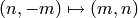 is invertible.
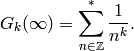
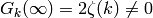
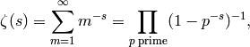
Proposition 2.2
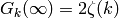 , where
  is the Riemann zeta
function.
is the Riemann zeta
function.
Proof
As  (along the imaginary axis) in (1),
the terms that involve with
(along the imaginary axis) in (1),
the terms that involve with  go to
go to  .
Thus
.
Thus
This sum is twice  ,
as claimed.
,
as claimed.
The Cusp Form 
Suppose  is an elliptic curve over
  , viewed as a
quotient of by a lattice
, viewed as a
quotient of by a lattice 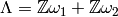 , with
 (see [DS05, Section 1.4]).
The Weierstrass
(see [DS05, Section 1.4]).
The Weierstrass  -function of
the lattice
-function of
the lattice  is
is
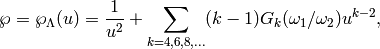
where the sum is over even integers .
It satisfies the differential equation

If we set  and
and  , the above is an (affine) equation of
the form
, the above is an (affine) equation of
the form 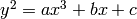 for an elliptic curve that is complex
analytically isomorphic to
for an elliptic curve that is complex
analytically isomorphic to  (see [Ahl78, pg. 277]
for why the cubic has distinct roots).
(see [Ahl78, pg. 277]
for why the cubic has distinct roots).
The discriminant of the cubic

is  , where

Since  is the difference of two modular forms of
weight it has weight . Morever,
is the difference of two modular forms of
weight it has weight . Morever,
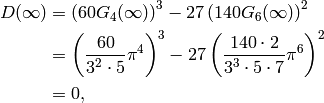
so  is a cusp form of weight .
Let

Lemma 2.3
If  , then
  .
.
Proof
Let  and
and  .
Since
.
Since  is an elliptic curve,
it has nonzero discriminant
is an elliptic curve,
it has nonzero discriminant
 .
.
Proposition 2.4
We have  .
.
Proof
See [Ser73, Thm. 6, pg. 95].
Remark 2.5
Sage computes the  -expansion of efficiently
to high precision using the command delta_qexp:
-expansion of efficiently
to high precision using the command delta_qexp:
sage: delta_qexp(6)
q - 24*q^2 + 252*q^3 - 1472*q^4 + 4830*q^5 + O(q^6)
Fourier Expansions of Eisenstein Series
Recall from (?) that elements  of
of  can be
expressed as formal power series in terms of
can be
expressed as formal power series in terms of  and
that this expansion is called the Fourier expansion of .
The following proposition gives the Fourier expansion of the
Eisenstein series .
and
that this expansion is called the Fourier expansion of .
The following proposition gives the Fourier expansion of the
Eisenstein series .
Definition 2.6
For any integer  and any positive integer
  ,
the sigma function
,
the sigma function
is the sum of the  powers of the positive divisors of .
Also, let
powers of the positive divisors of .
Also, let  , which is the number
of divisors of , and let
, which is the number
of divisors of , and let  .
For example, if
.
For example, if  is prime, then
  .
.
Proposition 2.7
For every even integer , we have
Proof
See [Ser73, Section VII.4], which uses clever manipulations of series, starting with the identity
From a computational point of view, the -expansion of
Proposition 2.7 is unsatisfactory because it involves
transcendental numbers. To understand these numbers, we introduce the
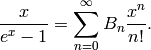
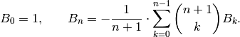
Bernoulli numbers  for
for  defined by the
following equality of formal power series:
defined by the
following equality of formal power series:
(2)
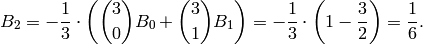
Expanding the power series, we have

As this expansion suggests, the Bernoulli numbers with  odd
are (see Exercise 2.2). Expanding the series further,
we obtain the following table:
odd
are (see Exercise 2.2). Expanding the series further,
we obtain the following table:


See Section Fast Computation of Bernoulli Numbers for a discussion of fast (analytic) methods for computing Bernoulli numbers.
We compute some Bernoulli numbers in Sage:
sage: bernoulli(12)
-691/2730
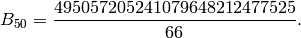
sage: bernoulli(50)
495057205241079648212477525/66
sage: len(str(bernoulli(10000)))
27706
A key fact is that Bernoulli numbers are
rational numbers and they are connected to values of at
positive even integers.
Proposition 2.8
If  is an even integer, then
Proof
This is proved
by manipulating a series expansion of  (see [Ser73, Section VII.4]).
Definition 2.9
The normalized Eisenstein series of even weight
is
Combining Proposition 2.7 and Proposition 2.8, we see that
(3)
Warning
Our series  is normalized so that the coefficient of
is , but often in the literature is normalized so that the
constant coefficient is . We use the normalization with the
coefficient of equal to , because then the eigenvalue of the
is normalized so that the coefficient of
is , but often in the literature is normalized so that the
constant coefficient is . We use the normalization with the
coefficient of equal to , because then the eigenvalue of the
 Hecke operator (see Section Hecke Operators) is the
coefficient of
Hecke operator (see Section Hecke Operators) is the
coefficient of  . Our normalization is also convenient when
considering congruences between cusp forms and Eisenstein series.
. Our normalization is also convenient when
considering congruences between cusp forms and Eisenstein series.
Structure Theorem for Level 1 Modular Forms
In this section we describe a structure theorem for modular
forms of level .
If is a nonzero meromorphic function on  and
and  , let
, let
 be the largest integer such that
  is
holomorphic at
is
holomorphic at  . If
. If  with
with
 , we set
  . We will use the following
theorem to give a presentation for the vector space of modular forms
of weight ; this presentation yields an algorithm
to compute this space.
. We will use the following
theorem to give a presentation for the vector space of modular forms
of weight ; this presentation yields an algorithm
to compute this space.
Let  denote the complex vector space of modular
forms of weight for
denote the complex vector space of modular
forms of weight for  . The
standard fundamental domain
. The
standard fundamental domain  for
is the set of
for
is the set of  with
with  and
and  . Let
. Let
 .
.
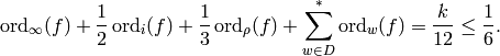
Theorem 2.11
Let be any integer and
suppose 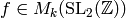 is nonzero. Then
where  is the sum over elements of
other than
is the sum over elements of
other than  and
and  !.
!.
Proof
The proof in [Ser73, Section VII.3] uses the residue theorem.
Let  index{
 }
denote the subspace of weight cusp forms for . We have
an exact sequence
}
denote the subspace of weight cusp forms for . We have
an exact sequence
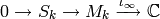
that sends  to
to  . When is even, the
space
. When is even, the
space  contains the Eisenstein series , and
 , so the map
  is surjective.
This proves the following lemma.
is surjective.
This proves the following lemma.
Lemma 2.12
If is even, then 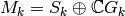 and the following sequence is exact:

Proposition 2.13
For  and
and  , we have
  .
.
Proof
Suppose is nonzero yet or . By
Theorem 2.11,
This is not possible because each quantity on the left is nonnegative so
whatever the sum is, it is too big (or , in which case  ).
).
Theorem 2.14
Multiplication by defines an isomorphism  .
.
Proof
By Lemma 2.3, is not identically , so
because is holomorphic, multiplication
by defines an injective map  .
To see that this map is surjective, we show that if
.
To see that this map is surjective, we show that if  , then
 .
Since has weight and
.
Since has weight and  ,
Theorem 2.11 implies that has a simple
zero at
,
Theorem 2.11 implies that has a simple
zero at  and does not vanish on .
Thus if and if we let
and does not vanish on .
Thus if and if we let  , then
  is holomorphic
and satisfies the appropriate transformation formula, so
is holomorphic
and satisfies the appropriate transformation formula, so  .
.
Corollary 2.15
For  , the space has dimension , with
basis ,
, the space has dimension , with
basis ,  ,
,  ,
,  ,
,  , and
, and  , respectively, and
 .
.
Proof
Combining Proposition 2.13 with
Theorem 2.14, we see that the spaces for
 cannot have dimension greater than , since otherwise
 for some
  . Also
  has dimension at most , since
 has dimension . Each of the indicated spaces of weight
 contains the indicated Eisenstein series and so has
dimension , as claimed.
contains the indicated Eisenstein series and so has
dimension , as claimed.
Corollary 2.16
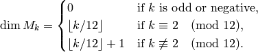
Here  is the biggest integer
  .
.
Proof
As we have already seen above, the formula is true when  .
By Theorem 2.14, the dimension increases by
when is replaced by
.
By Theorem 2.14, the dimension increases by
when is replaced by  .
.
Theorem 2.17
The space has as basis the modular forms  , where
 run over all pairs of nonnegative integers such that
 .
.
Proof
Fix an even integer . We first prove by induction that the
modular forms generate ; the cases and
 follow from the above arguments (e.g., when , we have
  and
basis ). Choose some pair of nonnegative integers
such that . The form
and
basis ). Choose some pair of nonnegative integers
such that . The form
 is not a cusp form, since it is nonzero at .
Now suppose is arbitrary. Since
is not a cusp form, since it is nonzero at .
Now suppose is arbitrary. Since  , there
exists
, there
exists  such that
  . Then by
Theorem 2.14, there is
. Then by
Theorem 2.14, there is  such that
  . By induction,
  is a polynomial in
and of the required type, and so is , so is
as well. Thus
is a polynomial in
and of the required type, and so is , so is
as well. Thus

spans .
Suppose there is a nontrivial linear relation between the  for a given . By multiplying the linear relation by a
suitable power of and , we may assume that we have
such a nontrivial relation with
for a given . By multiplying the linear relation by a
suitable power of and , we may assume that we have
such a nontrivial relation with  . Now divide the
linear relation by the weight form
. Now divide the
linear relation by the weight form  to see that
 satisfies a polynomial with coefficients in
(see Exercise 2.4). Hence
is a root of a polynomial, hence a constant, which is a
contradiction since the -expansion of is not
constant.
satisfies a polynomial with coefficients in
(see Exercise 2.4). Hence
is a root of a polynomial, hence a constant, which is a
contradiction since the -expansion of is not
constant.
Algorithm 2.18
Given integers and , this algorithm computes
a basis of -expansions for the complex vector
space mod . The -expansions output
by this algorithm have coefficients in  .
.
- [Simple Case] If , output the basis with just in it and
terminate; otherwise if
 or is odd, output the empty
basis and terminate.
or is odd, output the empty
basis and terminate. - [Power Series] Compute
 and
and  mod using the
formula from (3) and Section Fast Computation of Bernoulli Numbers.
mod using the
formula from (3) and Section Fast Computation of Bernoulli Numbers. - [Initialize] Set
 .
. - [Enumerate Basis] For each integer
 between and
 , compute
  .
If
.
If  is an integer, compute and output the basis
element
is an integer, compute and output the basis
element  . When computing
 , find
 for each
  , and save these
intermediate powers, so they can be reused later, and
likewise for powers of .
, and save these
intermediate powers, so they can be reused later, and
likewise for powers of .
Proof
This is simply a translation of Theorem 2.17
into an algorithm, since is a nonzero scalar multiple
of . That the -expansions have coefficients
in follows from (3).
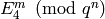
Example 2.19
We compute a basis for  , which is the space with
smallest weight whose dimension is greater than .
It has as basis
, which is the space with
smallest weight whose dimension is greater than .
It has as basis  ,
,  , and
, and  , whose explicit
expansions are
, whose explicit
expansions are
We compute this basis in Sage as follows:
sage: E4 = eisenstein_series_qexp(4, 3)
sage: E6 = eisenstein_series_qexp(6, 3)
sage: E4^6
1/191102976000000 + 1/132710400000*q
                  + 203/44236800000*q^2 + O(q^3)
sage: E4^3*E6^2
1/3511517184000 - 1/12192768000*q
                - 377/4064256000*q^2 + O(q^3)
sage: E6^4
1/64524128256 - 1/32006016*q + 241/10668672*q^2 + O(q^3)
In Section The Miller Basis, we will discuss the
reduced echelon form basis for .
The Miller Basis
Lemma 2.20
The space has a basis  such
that if
such
that if  is the
  coefficient of
  , then
 for
for  . Moreover
the all lie in
. Moreover
the all lie in ![\Z[[q]]](_images/math/30d204f5b49a5587d441b79d89f4914df9d5461a.png) . We call this basis the
Miller basis for .
. We call this basis the
Miller basis for .
This is a straightforward construction involving , and
. The following proof very closely follows
[Lan95, Ch. X,Thm. 4.4], which in turn follows the
first lemma of V. Miller’s thesis.
Proof
Let  . Since
  and
and  , we note that

and

have -expansions in with leading coefficient .
Choose integers  such that

with when , and let

Then it is elementary to check that  has weight

Hence the are linearly independent over , so form
a basis for . Since  , and are all in ,
so are the . The
, and are all in ,
so are the . The  may then be constructed from the
by Gauss elimination. The coefficients of the resulting power series lie in
may then be constructed from the
by Gauss elimination. The coefficients of the resulting power series lie in
 because each time we clear a column we use the power series
whose leading coefficient is (so no denominators are introduced).
because each time we clear a column we use the power series
whose leading coefficient is (so no denominators are introduced).
Remark 2.21
The basis coming from Miller’s lemma is “canonical”“,
since it is just the reduced row echelon form of any basis.
Also the set of all integral linear combinations of
the elements of the Miller basis are precisely
the modular forms of level with integral -expansion.
We extend the Miller basis to all by taking
a multiple of with constant term and subtracting
off the from the Miller basis so that the
coefficients of  of
the resulting expansion are . We call the extra basis
element
of
the resulting expansion are . We call the extra basis
element  .
.
Example 2.22
If  , then
  . Choose , since .
Then
. Choose , since .
Then

and

We let  and
and

Example 2.23
When  , the Miller basis including is
Example 2.24
The Sage command victor_miller_basis computes the Miller
basis to any desired precision given .
sage: victor_miller_basis(28,5)
[
1 + 15590400*q^3 + 36957286800*q^4 + O(q^5),
q + 151740*q^3 + 61032448*q^4 + O(q^5),
q^2 + 192*q^3 - 8280*q^4 + O(q^5)
]
Remark 2.25
To write  as a polynomial in and ,
it is wasteful to compute the Miller basis. Instead,
use the upper triangular (but not echelon!) basis
as a polynomial in and ,
it is wasteful to compute the Miller basis. Instead,
use the upper triangular (but not echelon!) basis  , and match coefficients from
  to
to  .
.
Hecke Operators
In this section we define Hecke operators on level modular forms and
derive their basic properties. We will not give proofs of the
analogous properties for Hecke operators on higher level modular
forms, since the proofs are clearest in the level case, and the
general case is similar (see, e.g., [Lan95]).
For any positive integer , let

Note that the set  is in bijection with the set of subgroups of
 of index , where
  corresponds to
 , as one can see using
Hermite normal form, which is the analogue over of
echelon form (see Exercise 7.5).
, as one can see using
Hermite normal form, which is the analogue over of
echelon form (see Exercise 7.5).
Recall from (?) that
if  , then
![f^{[\gamma]_k} = \det(\gamma)^{k-1} (cz+d)^{-k} f(\gamma(z)).](_images/math/bff7a83af850b2fdab4cb1b4e8046e96f6f77d5d.png)
Definition 2.26
The Hecke operator  of weight
is the operator on the set of functions on defined by
of weight
is the operator on the set of functions on defined by
![T_{n,k}(f) = \sum_{\gamma \in X_n}
f^{[\gamma]_k}.](_images/math/2975551bab9235dcc02d45318fe540c1837257ba.png)
Remark 2.27
It would make more sense to write on the right, e.g.,
 , since is defined using
a right group action.
However, if
, since is defined using
a right group action.
However, if  are integers, then the action of and
 on weakly modular functions commutes (by
Proposition 2.29 below), so it makes no difference
whether we view the Hecke operators of given weight as
acting on the right or left.
on weakly modular functions commutes (by
Proposition 2.29 below), so it makes no difference
whether we view the Hecke operators of given weight as
acting on the right or left.
Proposition 2.28
If is a weakly modular function of weight , then so is
 ; if is a modular function, then so is .
Proof
Suppose  . Since
  induces an automorphism of ,
X_n \cdot \gamma = \{ \delta \gamma : \delta\in X_n\}
is also in bijection with the subgroups
of of index .
For each element
induces an automorphism of ,
X_n \cdot \gamma = \{ \delta \gamma : \delta\in X_n\}
is also in bijection with the subgroups
of of index .
For each element  , there
is
, there
is  such that
  (the
element
(the
element  transforms
  to Hermite normal form),
and the set of elements
to Hermite normal form),
and the set of elements  is thus equal to .
Thus
is thus equal to .
Thus
![T_{n,k}(f) = \sum_{\sigma\delta\gamma\in X_n} f^{[\sigma\delta\gamma]_k}
= \sum_{\delta\in X_n} f^{[\delta\gamma]_k}
= T_{n,k}(f)^{[\gamma]_k}.](_images/math/e062631401777247317d291efa1866f952a4f144.png)
A finite sum of meromorphic function is
meromorphic, so is weakly modular.
If is holomorphic on , then
each ![f^{[\delta]_k}](_images/math/b4038f97856102c91ed970b75d1e4e69bda3dcac.png) is holomorphic on for
is holomorphic on for  .
A finite sum of holomorphic functions is holomorphic,
so is holomorphic.
.
A finite sum of holomorphic functions is holomorphic,
so is holomorphic.
We will frequently drop from the notation in , since
the weight is implicit in the modular function to which
we apply the Hecke operator. Henceforth we make the
convention that if we write  and if is modular,
then we mean , where is the weight of .
and if is modular,
then we mean , where is the weight of .
Proposition 2.29
On weight modular functions we have
(4)
and
(5)
Proof
Let  be a subgroup of index
  . The quotient
  is an
abelian group of order , and
is an
abelian group of order , and  , so decomposes
uniquely as a direct sum of a subgroup of order
, so decomposes
uniquely as a direct sum of a subgroup of order  with a subgroup of
order . Thus there exists a unique subgroup
with a subgroup of
order . Thus there exists a unique subgroup  such that
 , and has index in . The
subgroup corresponds to an element of
, and has index in . The
subgroup corresponds to an element of  , and the index
subgroup
, and the index
subgroup  corresponds to multiplying that element on
the right by some uniquely determined element of . We thus
have
corresponds to multiplying that element on
the right by some uniquely determined element of . We thus
have

i.e., the set products of elements in with elements of
equal the elements of  , up to -equivalence.
Thus for any , we have
, up to -equivalence.
Thus for any , we have
 . Applying this formula with and
swapped yields the equality
. Applying this formula with and
swapped yields the equality  .
.
We will show that  .
Suppose is a weight weakly modular function.
Using that
.
Suppose is a weight weakly modular function.
Using that
![f^{[\abcd{p}{0}{0}{p}]_k} = (p^2)^{k-1}p^{-k} f = p^{k-2} f](_images/math/a0c72b82e67f74ba14cb69254e42a41e2f04dd00.png) ,
we have
,
we have
![\sum_{x\in X_{p^n}} f^{[x]_k}\,\, +\,\, p^{k-1}\!\!\! \sum_{x\in
X_{p^{n-2}}} f^{[x]_k}
= \sum_{x\in X_{p^n}} f^{[x]_k} \,\,\,+\, p\!\!\!\! \sum_{x\in pX_{p^{n-2}}}
f^{[x]_k}.](_images/math/7c8f9950a3cfd59fa16b60111ce8315954949be6.png)
Also
![T_p T_{p^{n-1}}(f) = \sum_{y\in X_p} \sum_{x\in X_{p^{n-1}}}
(f^{[x]_k})^{[y]_k} = \sum_{x \in X_{p^{n-1}}\cdot X_p}
f^{[x]_k}.](_images/math/c9a5138e7976e44cedb64f4a91556a57ec24b5e0.png)
Thus it suffices to show that  disjoint union copies
of
disjoint union copies
of  is equal to
  , where we
consider elements with multiplicities and up to left
-equivalence (i.e., the left action of ).
, where we
consider elements with multiplicities and up to left
-equivalence (i.e., the left action of ).
Suppose is a subgroup of of index  , so
corresponds to an element of . First suppose is not
contained in
, so
corresponds to an element of . First suppose is not
contained in  . Then the image of in
  is of order , so if
  , then
![[\Z^2:L']=p](_images/math/622433093ac24748be582aaa4e6c33180dd595ac.png) and
and ![[L:L']=p^{n-1}](_images/math/88dfabd0870de05840df7d28f33609e3b01d3d3f.png) , and is the only subgroup
with this property. Second, suppose that
, and is the only subgroup
with this property. Second, suppose that  if of
index and that
if of
index and that  corresponds to . Then every
one of the
corresponds to . Then every
one of the  subgroups
  of index
contains . Thus there are chains
with .
of index
contains . Thus there are chains
with .
The chains  with and
![[\Z^2:L]=p^{n-1}](_images/math/342dacddc04c5b8e4d3a46dea8035f0b056ea7ef.png) are in bijection with the elements of
. On the other hand the union of with
copies of corresponds to the subgroups of index
are in bijection with the elements of
. On the other hand the union of with
copies of corresponds to the subgroups of index
 , but with those that contain counted times. The
structure of the set of chains that we
derived in the previous paragraph gives the result.
, but with those that contain counted times. The
structure of the set of chains that we
derived in the previous paragraph gives the result.
Corollary 2.30
The Hecke operator  , for prime , is a polynomial
in
, for prime , is a polynomial
in  with integer coefficients, i.e.,
 ![T_{p^n}\in\Z[T_p]](_images/math/14242ccaa8ee4a0a3d343e971ab3d103b0d148e6.png) .
If are any integers, then
.
If are any integers, then 
Proof
The first statement follows from (5) of
Proposition 2.29. It then follows that
when and are both powers of a single prime .
Combining this with (4) gives the second
statement in general.
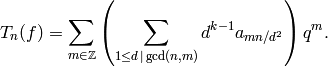
Proposition 2.31
Let  be a modular function
of weight .
Then
be a modular function
of weight .
Then
In particular, if  is prime, then
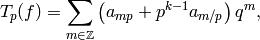
where  if
if  .
.
Proof
This is proved in [Ser73, Section VII.5.3] by writing
out  explicitly and using that
 is
is  if
if  and otherwise.
Corollary 2.32
The Hecke operators preserve and .
Remark 2.33
Alternatively, for the above corollary is
Proposition 2.28, and for we see from the
definitions that if  , then
  also vanishes
at .
also vanishes
at .
Example 2.34
Recall from (3) that

Using the formula of Proposition 2.31, we see that

Since  has dimension and since we have proved that
  preserves , we know that acts as a scalar. Thus
we know just from the constant coefficient of
preserves , we know that acts as a scalar. Thus
we know just from the constant coefficient of  that
that
More generally, for prime we see by inspection of
the constant coefficient of  that
that
In fact
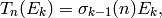
for any integer  and even weight .
Example 2.35
By Corollary Corollary 2.32, the Hecke operators  also
preserve the subspace of . Since
also
preserve the subspace of . Since  has dimension
(spanned by ), we see that is an eigenvector
for every . Since the coefficient of in the -expansion
of is , the eigenvalue of on is the
coefficient of . Since
has dimension
(spanned by ), we see that is an eigenvector
for every . Since the coefficient of in the -expansion
of is , the eigenvalue of on is the
coefficient of . Since  for
for  ,
we have proved the nonobvious fact that the
Ramanujan function
,
we have proved the nonobvious fact that the
Ramanujan function  that gives the
coefficient of is a multiplicative function, i.e.,
if , then
that gives the
coefficient of is a multiplicative function, i.e.,
if , then  .
.
Remark 2.36
The Hecke operators respect the decomposition
 , i.e., for all the series are
eigenvectors for all .
, i.e., for all the series are
eigenvectors for all .
Computing Hecke Operators
This section is about how to compute matrices
of Hecke operators on .
Algorithm 2.37
This algorithm computes the matrix of the Hecke operator on the
Miller basis for .
[Dimension] Compute
 using
Corollary 2.16.
using
Corollary 2.16.[Basis] Using Lemma 2.20, compute the echelon basis
 for
for  .
.[Hecke operator] Using Proposition 2.31, compute for each
the image  .
.[Write in terms of basis] The elements
 determine linear combinations of
These linear combinations are easy to find once we compute
, since our basis of is in
echelon form. The linear combinations are just the coefficients
of the power series  up to and including .
[Write down matrix] The matrix of
acting from the right
relative to the basis  is the matrix whose
rows are the linear combinations found in the previous step,
i.e., whose rows are the coefficients of .
is the matrix whose
rows are the linear combinations found in the previous step,
i.e., whose rows are the coefficients of .
Proof
By Proposition 2.31, the  coefficient
of involves only
coefficient
of involves only  and smaller-indexed coefficients
of . We need only compute a modular form modulo
and smaller-indexed coefficients
of . We need only compute a modular form modulo  in
order to compute modulo
in
order to compute modulo  .
Uniqueness in step (4) follows from Lemma 2.20
above.
.
Uniqueness in step (4) follows from Lemma 2.20
above.
Example 2.38
We compute the Hecke operator on  using the above
algorithm.
using the above
algorithm.
[Compute dimension] We have
 .
.[Compute basis] Compute up to (but not including) the coefficient of
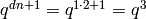 . As given in
the proof of Lemma 2.20, we have
. As given in
the proof of Lemma 2.20, we have
Thus $M_{12}$ has basis

Sage does the arithmetic in the above calculation as follows:
sage: R.<q> = QQ[['q']]
sage: F4 =  240 * eisenstein_series_qexp(4,3)
sage: F6 = -504 * eisenstein_series_qexp(6,3)
sage: F4^3
1 + 720*q + 179280*q^2 + O(q^3)
sage: Delta = (F4^3 - F6^2)/1728; Delta
q - 24*q^2 + O(q^3)
sage: F4^3 - 720*Delta
1 + 196560*q^2 + O(q^3)
[Compute Hecke operator] In each case letting
 denote
the coefficient of or
denote
the coefficient of or  , respectively, we
have
, respectively, we
have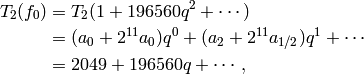
and
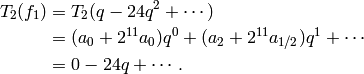
(Note that
 .)
.)[Write in terms of basis] We read off at once that

[Write down matrix] Thus the matrix of
, acting from the
right on the basis , , is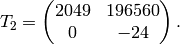
As a check note that the characteristic polynomial of is
 and that
  is the sum of the
 powers of the divisors of
  .
.
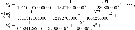
Example 2.39
The Hecke operator on  with respect to the echelon
basis is
with respect to the echelon
basis is
It has characteristic polynomial

where the cubic factor is irreducible.
The echelon_form command creates the space of modular forms but with basis in echelon form (which is not the default).
sage: M = ModularForms(1,36, prec=6).echelon_form()
sage: M.basis()
[
1 + 6218175600*q^4 + 15281788354560*q^5 + O(q^6),
q + 57093088*q^4 + 37927345230*q^5 + O(q^6),
q^2 + 194184*q^4 + 7442432*q^5 + O(q^6),
q^3 - 72*q^4 + 2484*q^5 + O(q^6)
]
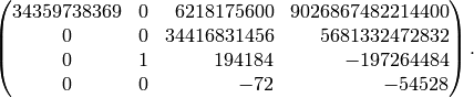
Next we compute the matrix of the Hecke operator .
sage: T2 = M.hecke_matrix(2); T2
[34359738369   0       6218175600 9026867482214400]
[          0   0      34416831456    5681332472832]
[          0   1           194184       -197264484]
[          0   0              -72           -54528]
Finally we compute and factor its characteristic polynomial.
sage: T2.charpoly().factor()
(x - 34359738369) * (x^3 - 139656*x^2 - 59208339456*x - 1467625047588864)
The following is a famous open problem about Hecke operators on
modular forms of level . It generalizes our above observation that
the characteristic polynomial of on , for  ,
factors as a product of a linear factor and an irreducible factor.
,
factors as a product of a linear factor and an irreducible factor.
Conjuecture 2.40
The characteristic polynomial of on is irreducible for
any .
Kevin Buzzard observed that in several specific cases the Galois group of
the characteristic polynomial of is the full symmetric group
(see [Buz96]). See also [FJ02] for more
evidence for the following conjecture:
Conjuecture 2.41
For all primes and all even the characteristic
polynomial of  acting on is irreducible.
Fast Computation of Fourier Coefficients
How difficult is it to compute prime-indexed coefficients of

Theorem 2.42
Let be a prime. There is a probabilistic algorithm to compute
 , for prime , that has expected running time polynomial
in
, for prime , that has expected running time polynomial
in 
Proof
See [ECdJ+06].
More generally, if  is an eigenform in some space
 , where , then one expects that there is an
algorithm to compute
, where , then one expects that there is an
algorithm to compute  in time polynomial in . Bas
Edixhoven, Jean-Marc Couveignes and Robin de Jong have proved that
can be computed in polynomial time; their approach involves
sophisticated techniques from arithmetic geometry (e.g., ‘etale
cohomology, motives, Arakelov theory). The ideas they use are inspired
by the ones introduced by Schoof, Elkies and Atkin for quickly
counting points on elliptic curves over finite fields (see
[Sch95]).
in time polynomial in . Bas
Edixhoven, Jean-Marc Couveignes and Robin de Jong have proved that
can be computed in polynomial time; their approach involves
sophisticated techniques from arithmetic geometry (e.g., ‘etale
cohomology, motives, Arakelov theory). The ideas they use are inspired
by the ones introduced by Schoof, Elkies and Atkin for quickly
counting points on elliptic curves over finite fields (see
[Sch95]).
Edixhoven describes (in an email to the author) the strategy as follows:
- We compute the mod
 Galois representation associated
to . In particular, we produce a polynomial such that
Galois representation associated
to . In particular, we produce a polynomial such that
![\Q[x]/(f)](_images/math/a27f547d7ccef1a3d0d72faf6ea89c499211f71a.png) is the fixed field of
is the fixed field of  . This is then used
to obtain
. This is then used
to obtain  and to do a Schoof-like algorithm
for computing .
and to do a Schoof-like algorithm
for computing . - We compute the field of definition of suitable points of
order on the modular Jacobian
 to do part (1) (see
[DS05, Ch. 6] for the definition of ).
to do part (1) (see
[DS05, Ch. 6] for the definition of ). - The method is to approximate the polynomial in some sense
(e.g., over the complex numbers or modulo many small primes
 )
and to use an estimate from Arakelov theory to determine a
precision that will suffice.
)
and to use an estimate from Arakelov theory to determine a
precision that will suffice.
Fast Computation of Bernoulli Numbers
This section, which was written jointly with Kevin McGown, is about
computing the Bernoulli numbers , for , defined in
Section Fourier Expansions of Eisenstein Series by
(6)
One way to compute is to multiply both sides of
(?) by  and equate coefficients of
 to obtain the recurrence
This recurrence provides a straightforward and easy-to-implement
method for calculating if one is interested in
computing for all up to some bound.
For example,
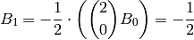
and
However, computing via the recurrence is slow; it requires
summing over many large terms, it requires storing the numbers
 , and it takes only limited advantage of
asymptotically fast arithmetic algorithms. There is also an inductive
procedure to compute Bernoulli numbers that resembles Pascal’s
triangle called the Akiyama-Tanigawa algorithm (see
[Kan00]).
, and it takes only limited advantage of
asymptotically fast arithmetic algorithms. There is also an inductive
procedure to compute Bernoulli numbers that resembles Pascal’s
triangle called the Akiyama-Tanigawa algorithm (see
[Kan00]).
Another approach to computing is to use Newton
iteration and asymptotically fast polynomial arithmetic to approximate
 . This method yields a very fast algorithm to compute
 modulo .
See [BCS92] for an application of this
method modulo a prime to the verification of
Fermat’s last theorem for irregular primes up to one million.
modulo .
See [BCS92] for an application of this
method modulo a prime to the verification of
Fermat’s last theorem for irregular primes up to one million.
Example 2.43
David Harvey implemented the algorithm of [BCS92] in Sage as the command bernoulli_mod_p:
sage: bernoulli_mod_p(23)
[1, 4, 13, 17, 13, 6, 10, 5, 10, 9, 15]
A third way to compute uses
an algorithm based on Proposition 2.8,
which we explain below (Algorithm 2.45).
This algorithm appears to
have been independently invented by several people: by Bernd C.
Kellner (see [Kel06]); by Bill Dayl; and by H. Cohen and
K. Belabas.
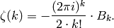
We compute as an exact rational number
by approximating  to very high precision using
Proposition 2.8, the
Euler product
to very high precision using
Proposition 2.8, the
Euler product
and the following theorem:
Theorem 2.44
For even  ,
,
Proof
See [Lan95, Ch. X, Thm. 2.1].
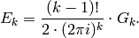
The Number of Digits of 
The following is a new quick way to compute the number of digits of
the numerator of . For example, using it we can compute the
number of digits of  in less than a second.
By Theorem 2.44 we have
 . The number of digits of
the numerator is thus
. The number of digits of
the numerator is thus
But
and  so
so  .
Finally, Stirling’s formula (see [Ahl78, pg. 198–206])
gives a fast way to compute
.
Finally, Stirling’s formula (see [Ahl78, pg. 198–206])
gives a fast way to compute  :
:
(7)
We put quotes around the equality sign because  does
not converge to its Laurent series. Indeed, note that for any fixed
value of the summands on the right side go to as
does
not converge to its Laurent series. Indeed, note that for any fixed
value of the summands on the right side go to as
 ! Nonetheless, we can use this formula to very efficiently
compute , since if we truncate the sum, then the
error is smaller than the next term in the infinite sum.
! Nonetheless, we can use this formula to very efficiently
compute , since if we truncate the sum, then the
error is smaller than the next term in the infinite sum.
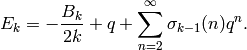
Computing Exactly
We return to the problem of computing . Let

so  . Write

with  ,
,  , and
, and  .
It is elementary
to show that
.
It is elementary
to show that  for even .
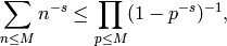
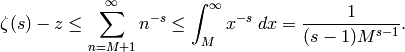
Suppose that using the Euler product we approximate
from below by a number such that
for even .
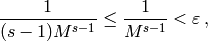
Suppose that using the Euler product we approximate
from below by a number such that
Then  hence
hence  It follows that
  and hence
It remains to compute .
Consider the following problem:
given  and
and
 , find
  so that
satisfies  .
We always have
.
We always have  .
Also,
.
Also,
so
Thus if 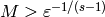 , then
so  , as required.
For our purposes, we have
, as required.
For our purposes, we have  and
and  ,
so it suffices to take
,
so it suffices to take  .
.
Algorithm 2.45
Given an integer , this algorithm computes
the Bernoulli number as an exact rational number.
- [Special cases] If
 , return ; if
  , return
  ;
if
;
if  is odd, return .
 - [Factorial factor] Compute
 to sufficiently many digits of precision so
the ceiling in step (6) is uniquely determined
(this precision can be determined using
Section The Number of Digits of ).
to sufficiently many digits of precision so
the ceiling in step (6) is uniquely determined
(this precision can be determined using
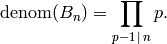
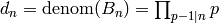
Section The Number of Digits of ). - [Denominator] Compute
 .
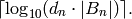
. - [Bound] Compute
- [Approximate ] Compute
 .
. - [Numerator] Compute
 .
. - [Output ] Return
 .
.
In step (5) use a sieve to compute all primes
 efficiently (which is fast, since
  is so small). In
step (4) we may replace by any integer greater
than the one specified by the formula, so we do not have to compute
is so small). In
step (4) we may replace by any integer greater
than the one specified by the formula, so we do not have to compute
 to very high precision.
In Section Computing Generalized Bernoulli Numbers Analytically below we will generalize the above algorithm.
Example 2.46
We illustrate Algorithm 2.45 by computing  .
Using 135 binary digits of precision, we compute
.
Using 135 binary digits of precision, we compute

The divisors of are  , so
, so

We find  and compute

Finally we compute

so
Exercises
Exercise 2.1
Using Proposition 2.8 and the table found here, compute
 explicitly.
Exercise 2.2
Prove that if is odd, then the Bernoulli number is .
Exercise 2.3
Use (3) to write down the coefficients of , ,
 , and
, and  of the Eisenstein series
  .
.
Exercise 2.4
Suppose is a positive integer with  .
Suppose are integers with
.
Suppose are integers with  .
.
- Prove
 .
. - Show that
Exercise 2.5
Compute the Miller basis for  with precision
 . Your answer will look like Example 2.23.
Exercise 2.6
Consider the cusp form  in
in
 . Write as a polynomial in and
(see Remark 2.25).
. Write as a polynomial in and
(see Remark 2.25).
Exercise 2.7
Let be the weight Eisenstein series from
equation (1). Let  be the complex number so that the
constant coefficient of the -expansion of
be the complex number so that the
constant coefficient of the -expansion of  is . Is it always the case that the -expansion of lies
in ?
is . Is it always the case that the -expansion of lies
in ?
Exercise 2.8
Compute the matrix of the Hecke operator on the Miller basis
for  . Then compute its characteristic
polynomial and verify it factors as a product of two irreducible
polynomials.
. Then compute its characteristic
polynomial and verify it factors as a product of two irreducible
polynomials.
What Next? Much of the rest of this book is about methods for
computing subspaces of for general  and .
These general methods are more complicated than the methods presented
in this chapter, since there are many more modular forms of small
weight and it can be difficult to obtain them. Forms of level
and .
These general methods are more complicated than the methods presented
in this chapter, since there are many more modular forms of small
weight and it can be difficult to obtain them. Forms of level  have subtle connections with elliptic curves, abelian varieties, and
motives. Read on for more!
have subtle connections with elliptic curves, abelian varieties, and
motives. Read on for more!
Table Of Contents
- Modular Forms of Level 1