Dimension Formulas
When computing with spaces of modular forms, it is helpful to have
easy-to-compute formulas for dimensions of these spaces. Such
formulas provide a check on the output of the algorithms from
Chapter General Modular Symbols that compute explicit bases for spaces of
modular forms. We can also use dimension formulas to improve the
efficiency of some of the algorithms in Chapter General Modular Symbols, since
we can use them to determine the ranks of certain matrices without
having to explicitly compute those matrices. Dimension formulas can also be
used in generating bases of  -expansions; if we know the dimension
of
-expansions; if we know the dimension
of  and if we have a process for computing -expansions
of elements of , e.g., multiplying together
-expansions of certain forms of smaller weight, then we can tell
when we are done generating .
and if we have a process for computing -expansions
of elements of , e.g., multiplying together
-expansions of certain forms of smaller weight, then we can tell
when we are done generating .
This chapter contains formulas for dimensions of spaces of modular forms, along with some remarks about how to evaluate these formulas. In some cases we give dimension formulas for spaces that we will define in later chapters. We also give many examples, some of which were computed using the modular symbols algorithms from Chapter General Modular Symbols.
Many of the dimension formulas and algorithms we give below grew out of Shimura’s book [Shi94] and a program that Bruce Kaskel wrote (around 1996) in PARI, which Kevin Buzzard extended. That program codified dimension formulas that Buzzard and Kaskel found or extracted from the literature (mainly [Shi94, Section 2.6]). The algorithms for dimensions of spaces with nontrivial character are from [CO77], with some refinements suggested by Kevin Buzzard.
For the rest of this chapter,  denotes a positive integer and
 is an integer. We will give no simple formulas for
dimensions of spaces of weight
is an integer. We will give no simple formulas for
dimensions of spaces of weight  modular forms; in fact, it
might not be possible to give such formulas since the
methods used to derive the formulas below do not apply in the case
modular forms; in fact, it
might not be possible to give such formulas since the
methods used to derive the formulas below do not apply in the case
 . If
. If  , the only modular forms are the constants, and for
 the dimension of is
  .
.
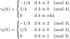
For a nonzero integer and a prime  , let
, let  be the largest
integer
be the largest
integer  such that
  . In the formulas in this
chapter, always denotes a prime number. Let be the
space of modular forms of level weight
. In the formulas in this
chapter, always denotes a prime number. Let be the
space of modular forms of level weight  and character
  ,
and let
,
and let  and
and  be the cuspidal and Eisenstein
subspaces, respectively.
be the cuspidal and Eisenstein
subspaces, respectively.
The dimension formulas below for  ,
,
 ,
,  and
and  can be
found in [DS05, Ch. 3],
[Shi94, Section 2.6] [1] and
[Miy89, Section 2.5]. They are derived using the Riemann-Roch Theorem
applied to the covering
can be
found in [DS05, Ch. 3],
[Shi94, Section 2.6] [1] and
[Miy89, Section 2.5]. They are derived using the Riemann-Roch Theorem
applied to the covering  or
or  and
appropriately chosen divisors. It would be natural to give a sample
argument along these lines at this point, but we will not since it
easy to find such arguments in other books and survey papers (see,
e.g., [DI95]). So you will not learn much about how to
derive dimension formulas from this chapter. What you will learn is
precisely what the dimension formulas are, which is something that is
often hard to extract from obscure references.
and
appropriately chosen divisors. It would be natural to give a sample
argument along these lines at this point, but we will not since it
easy to find such arguments in other books and survey papers (see,
e.g., [DI95]). So you will not learn much about how to
derive dimension formulas from this chapter. What you will learn is
precisely what the dimension formulas are, which is something that is
often hard to extract from obscure references.
In addition to reading this chapter, the reader may wish to consult [Mar05] for proofs of similar dimension formulas, asymptotic results, and a nonrecursive formula for dimensions of certain new subspaces.
Modular Forms for  
For any prime and any positive integer , let be
the power of that divides . Also, let
Note that  is the index of in
  (see Exercise 6.1).
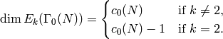
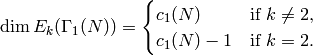
Proposition 6.1
We have  , and
for
, and
for  even,
even,
The dimension of the Eisenstein subspace is
The following is a table of 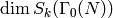 for some values of and :
Example 6.2
Use the commands dimension_cusp_forms,
dimension_eis, and dimension_modular_forms
to compute the dimensions of the three spaces ,
and  , respectively.
For example,
, respectively.
For example,
sage: dimension_cusp_forms(Gamma0(2007),2)
221
sage: dimension_eis(Gamma0(2007),2)
7
sage: dimension_modular_forms(Gamma0(2007),2)
228
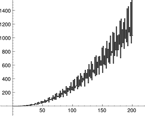
Remark 6.3
Csirik, Wetherell, and Zieve prove in
[CWZ01] that a random positive integer has
probability of being a value of

and they give bounds on the size of the set of values of  below
some given
below
some given  . For example, they show that
  are the first few integers that are not of the
form for any . See Figure 6.1
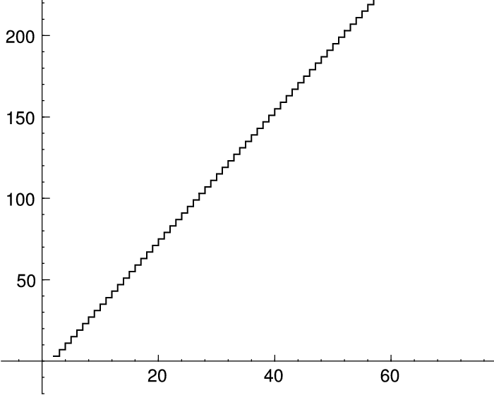
for a plot of the very erratic function . In
contrast, the function
are the first few integers that are not of the
form for any . See Figure 6.1
for a plot of the very erratic function . In
contrast, the function  is very
well behaved (see Figure 6.2).
is very
well behaved (see Figure 6.2).
Figure 6.1
Dimension of  as a function of
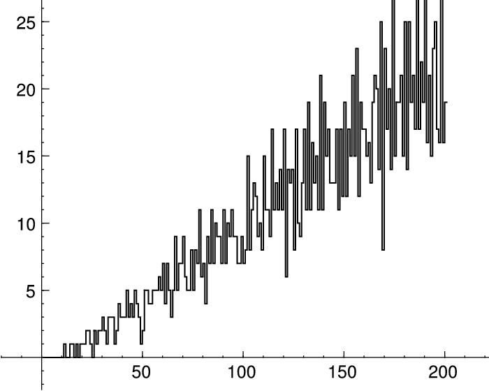
Figure 6.2
Dimension of  as a function of .
New and Old Subspaces
In this section we assume the reader is either familiar with newforms or has read Section Atkin-Lehner-Li Theory.
For any integer  , let
, let
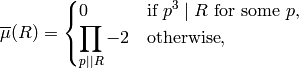
where the product is over primes that exactly divide .
Note that  is not the Moebius function, but it
has a similar flavor.
is not the Moebius function, but it
has a similar flavor.
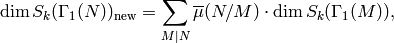
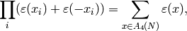
Proposition 6.4
The dimension of the new subspace is

where the sum is over the positive divisors  of .
As a consequence of Theorem 9.4,
we also have
of .
As a consequence of Theorem 9.4,
we also have
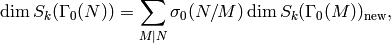
where  is the number of divisors of
  .
.
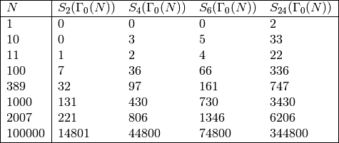
Example 6.5
We compute the dimension of the new subspace of
using the Sage command dimension_new_cusp_forms
as follows:
sage: dimension_new_cusp_forms(Gamma0(11),12)
8
sage: dimension_cusp_forms(Gamma0(11),12)
10
sage: dimension_new_cusp_forms(Gamma0(2007),12)
1017
sage: dimension_cusp_forms(Gamma0(2007),12)
2460
Modular Forms for  
This section follows Section Modular Forms for closely, but with
suitable modifications with replaced by .
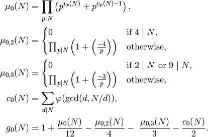
Define functions of a positive integer by the following formulas:
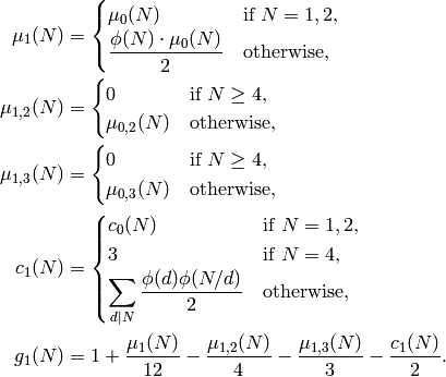
Note that  is the genus of the modular curve
  (associated
to ) and
(associated
to ) and  is the number of cusps of .
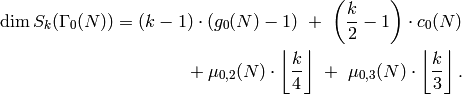
Proposition 6.6
We have  . If
. If  , then
 so
so

where is given by the formula of
Proposition 6.1. If  , let
, let
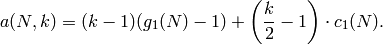
Then for  ,
,
The dimension of the Eisenstein subspace is as follows:
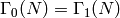
The dimension of the new subspace of  is
is
where is as in the statement
of Proposition 6.4.
Remark 6.7
Since 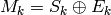 , the formulas above for
 and
and  also yield
a formula for the dimension of
also yield
a formula for the dimension of  .
.
Figure 6.3
Dimension of  as a function of .
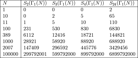
The following table contains the dimension of
for some sample values of and :
Example 6.8
We compute dimensions of spaces of modular forms for :
sage: dimension_cusp_forms(Gamma1(2007),2)
147409
sage: dimension_eis(Gamma1(2007),2)
3551
sage: dimension_modular_forms(Gamma1(2007),2)
150960
Modular Forms with Character
Fix a Dirichlet character of modulus ,
and let  be the conductor of (we do not
assume that is primitive).
Assume that
be the conductor of (we do not
assume that is primitive).
Assume that  , since otherwise
 and the formulas of
Section Modular Forms for apply. Also, assume that
and the formulas of
Section Modular Forms for apply. Also, assume that  ,
since otherwise
,
since otherwise  . In this section we
discuss formulas for computing each of ,
and .
. In this section we
discuss formulas for computing each of ,
and .
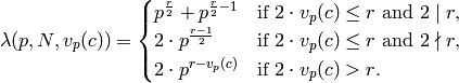
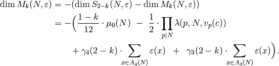
In [CO77], Cohen and
Oesterl’e assert (without published proof; see Remark Remark 6.11 below)
that for any  and ,
as above,
and ,
as above,
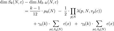
where is as in Section Modular Forms for ,
 and
and
 ,
and
,
and  are
are
It remains to define  .
Fix a prime divisor
.
Fix a prime divisor  and let
  .
Then
.
Then
This flexible formula can be used to compute the dimension of
,
, and for any , ,  ,
by using that
,
by using that
One thing that is not straightforward when implementing an algorithm
to compute the above dimension formulas is how to efficiently compute
the sets  and
and  . Kevin Buzzard suggested the
following two algorithms. Note that if
is odd, then
. Kevin Buzzard suggested the
following two algorithms. Note that if
is odd, then  , so the sum over
is only needed when is even.
, so the sum over
is only needed when is even.
Algorithm 6.9
Given a positive integer and an even
Dirichlet character of modulus ,
this algorithm computes  .
.
[Factor
] Compute the prime factorization
 of .
of .[Initialize] Set
 and
and  .
.[Loop Over Prime Divisors] Set
 .
If
.
If  , return
  . Otherwise set
  and
and
 .
.- If
 , return .
 - If
 and
and  , return .
 - If and
 , go to step (3).
 - Compute a generator
 using
Algorithm 4.4.
using
Algorithm 4.4. - Compute
 .
. - Use the Chinese Remainder Theorem to find
 such that
  and
and  .
. - Set
 .
. - Set
 .
.
- If
 , set
, set  and go to
step (3).
and go to
step (3).
- If
 , set
, set  and go to
step (3).
and go to
step (3).
- If
Proof
Note that  , since is even. By the Chinese
Remainder Theorem, the set is empty if and only if there is
no square root of
, since is even. By the Chinese
Remainder Theorem, the set is empty if and only if there is
no square root of  modulo some prime power divisor of . If
is empty, the algorithm correctly detects this fact in
steps (a) – (b).
Thus assume is
nonempty. For each prime power
modulo some prime power divisor of . If
is empty, the algorithm correctly detects this fact in
steps (a) – (b).
Thus assume is
nonempty. For each prime power  that exactly divides
, let
that exactly divides
, let  be such that
  and
and  for
for  . This is the value of
computed in steps (d) – (g)
(as one sees using elementary number theory).
. This is the value of
computed in steps (d) – (g)
(as one sees using elementary number theory).
The next key observation is that
(1)
since by the Chinese Remainder Theorem the elements of are
in bijection with the choices for a square root of modulo each
prime power divisors of . The observation (1)
is a huge gain from an efficiency point of view—if had  prime factors, then would have size
  , which could be
prohibitive, where the product involves only factors. To finish
the proof, just note that steps
(h) – (j)
compute the local factors
, which could be
prohibitive, where the product involves only factors. To finish
the proof, just note that steps
(h) – (j)
compute the local factors  ,
where again we use that is even. Note that a solution
of
,
where again we use that is even. Note that a solution
of  lifts uniquely to a solution mod
  for
any
for
any  , because the kernel of the natural homomorphism
  is a group of -power order.
The algorithm for computing the sum over  is similar.
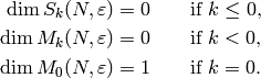
For , to compute  , use the formula directly
and the fact that
, use the formula directly
and the fact that  , unless
  and
and  .
To compute
.
To compute  for , use the fact that the big
formula at the beginning of this section
is valid for any integer to replace
by
for , use the fact that the big
formula at the beginning of this section
is valid for any integer to replace
by  and
that
and
that  for
for  to rewrite the formula as
Note also that for ,  if
and only if is trivial and it equals otherwise.
We then also obtain
if
and only if is trivial and it equals otherwise.
We then also obtain

We can also compute  when
directly, since
when
directly, since

The following table contains the dimension of
for some sample values of and . In each case,
is the product of characters  of maximal order
corresponding to the prime power factors of (i.e.,
the product of the generators of the group
of maximal order
corresponding to the prime power factors of (i.e.,
the product of the generators of the group
 of Dirichlet characters of modulus ).
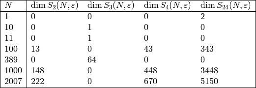
Example 6.10
We compute the last line of the above table. First
we create the character .
sage: G = DirichletGroup(2007)
sage: e = prod(G.gens(), G(1))
Next we compute the dimension of the four spaces.
sage: dimension_cusp_forms(e,2)
222
sage: dimension_cusp_forms(e,3)
0
sage: dimension_cusp_forms(e,4)
670
sage: dimension_cusp_forms(e,24)
5150
We can also compute dimensions of the corresponding spaces of Eisenstein series.
sage: dimension_eis(e,2)
4
sage: dimension_eis(e,3)
0
sage: dimension_eis(e,4)
4
sage: dimension_eis(e,24)
4
Remark 6.11
Cohen and Oesterl’e also give dimension formulas for spaces of
half-integral weight modular forms, which we do not give in this
chapter. Note that [CO77] does not
contain any proofs that their claimed formulas are correct,
but instead they say only that “Les formules qui les donnent sont
connues de beaucoup de gens et il existe plusieurs m’ethodes
permettant de les obtenir (th’eor`eme de Riemann-Roch, application
des formules de trace donn’ees par Shimura).” [2]
Fortunately, in [Que06],
Jordi Quer derives the
(integral weight) formulas of [CO77]
along with formulas for dimensions of spaces  and
and
 for more general congruence subgroups.
Let  be the conductor of a Dirichlet character of modulus .
Then the dimension of the new subspace of is
be the conductor of a Dirichlet character of modulus .
Then the dimension of the new subspace of is

where is as in the statement
of Proposition 6.4, and  is the restriction
of mod .
is the restriction
of mod .
Example 6.12
We compute the dimension of  for a quadratic character of modulus
  .
.
sage: G = DirichletGroup(2007, QQ)
sage: e = prod(G.gens(), G(1))
sage: dimension_new_cusp_forms(e,2)
76
Exercises
Exercise 6.1
Let  and
and  be as in this chapter.
- Prove that
![\mu_0(N) = [\SL_2(\Z):\Gamma_0(N)]](_images/math/aaeeb88680491cd95f63f7d19defb0c7cebaf2f3.png) .
. - Prove that for ,
![\mu_1(N) = [\SL_2(\Z):\Gamma_1(N)]/2](_images/math/0e4537e50b92631658a8397b7ec3cd1b32975b45.png) ,
so
,
so  is the index of
  in
in  .
.
Exercise 6.2
Use Proposition 6.4 to find a formula
for  . Verify that this formula is
the same as the one in Corollary Corollary 2.16.
. Verify that this formula is
the same as the one in Corollary Corollary 2.16.
Exercise 6.3
Suppose either that  or that is prime and .
Prove that
or that is prime and .
Prove that  .
.
Exercise 6.4
Fill in the details of the proof of Algorithm 6.9.
Exercise 6.5
Implement a computer program to compute
Footnotes
| [1] | The formulas in [Shi94, Section 2.6] contain some minor mistakes. |
| [2] | The formulas that we give here are well known and there exist many methods to prove them, e.g., the Riemann-Roch theorem and applications of the trace formula of Shimura. |
Table Of Contents
Previous topic
Eisenstein Series and Bernoulli Numbers