Computing in Higher Rank
by Paul E. Gunnells
A.1 Introduction
This book has addressed the theoretical and practical problems of
performing computations with modular forms. Modular forms are the
simplest examples of the general theory of automorphic forms attached
to a reductive algebraic group  with an arithmetic
subgroup
with an arithmetic
subgroup  ; they are the case
  with a
congruence subgroup of
with a
congruence subgroup of  . For such pairs
  the Langlands philosophy asserts that there should be deep connections
between automorphic forms and arithmetic, connections that are
revealed through the action of the Hecke operators on spaces of
automorphic forms. There have been many profound advances in recent
years in our understanding of these phenomena, for example:
the Langlands philosophy asserts that there should be deep connections
between automorphic forms and arithmetic, connections that are
revealed through the action of the Hecke operators on spaces of
automorphic forms. There have been many profound advances in recent
years in our understanding of these phenomena, for example:
- the establishment of the modularity of
elliptic curves defined over
 [Wil95, TW95, Dia96, CDT99, BCDT01],
 - the proof by Harris–Taylor of the local Langlands correspondence [HT01], and
- Lafforgue’s proof of the global Langlands correspondence for function fields [Laf02].
Nevertheless, we are still far from seeing that the links between automorphic forms and arithmetic hold in the broad scope in which they are generally believed. Hence one has the natural problem of studying spaces of automorphic forms computationally.
The goal of this appendix is to describe some computational techniques
for automorphic forms. We focus on the case  and
and
 , since the automorphic forms that arise
are one natural generalization of modular forms, and since this is the
setting for which we have the most tools available. In fact, we do not
work directly with automorphic forms, but rather with the cohomology
of the arithmetic group with certain coefficient modules.
This is the most natural generalization of the tools developed in
previous chapters.
, since the automorphic forms that arise
are one natural generalization of modular forms, and since this is the
setting for which we have the most tools available. In fact, we do not
work directly with automorphic forms, but rather with the cohomology
of the arithmetic group with certain coefficient modules.
This is the most natural generalization of the tools developed in
previous chapters.
Here is a brief overview of the contents. Section A.2 Automorphic Forms and Arithmetic Groups
gives background on automorphic forms and the cohomology of arithmetic
groups and explains why the two are related. In Section
A.3 Combinatorial Models for Group Cohomology we describe the basic topological tools used to
compute the cohomology of explicitly. Section
A.4 Hecke Operators and Modular Symbols defines the Hecke operators, describes the
generalization of the modular symbols from Chapter General Modular Symbols to
higher rank, and explains how to compute the action of the Hecke
operators on the top degree cohomology group. Section
A.5 Other Cohomology Groups discusses computation of the Hecke action on
cohomology groups below the top degree. Finally, Section A.6 Complements and Open Problems
briefly discusses some related material and presents some open
problems.
A.1.1
The theory of automorphic forms is notorious for the difficulty of its prerequisites. Even if one is only interested in the cohomology of arithmetic groups—a small part of the full theory—one needs considerable background in algebraic groups, algebraic topology, and representation theory. This is somewhat reflected in our presentation, which falls far short of being self-contained. Indeed, a complete account would require a long book of its own. We have chosen to sketch the foundational material and to provide many pointers to the literature; good general references are [BW00, Harb, Lab90, Vog97]. We hope that the energetic reader will follow the references and fill many gaps on his/her own.
The choice of topics presented here is heavily influenced (as usual) by the author’s interests and expertise. There are many computational topics in the cohomology of arithmetic groups we have completely omitted, including the trace formula in its many incarnations [GP05], the explicit Jacquet–Langlands correspondence [Dem04, SW05], and moduli space techniques [FvdG, vdG]. We encourage the reader to investigate these extremely interesting and useful techniques.
A.1.2 Acknowledgements
I thank Avner Ash, John Cremona, Mark McConnell, and Dan Yasaki for helpful comments. I also thank the NSF for support.
A.2 Automorphic Forms and Arithmetic Groups
A.2.1
Let 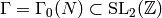 be the usual Hecke
congruence subgroup of matrices upper-triangular mod
be the usual Hecke
congruence subgroup of matrices upper-triangular mod  . Let
. Let
 be the modular curve
  , and let
 be its canonical compactification obtained by adjoining
cusps. For any integer
be its canonical compactification obtained by adjoining
cusps. For any integer  , let
, let  be the space of
weight
be the space of
weight  holomorphic cuspidal modular forms on . According
to Eichler–Shimura [Shi94, Chapter 8], we have the isomorphism
holomorphic cuspidal modular forms on . According
to Eichler–Shimura [Shi94, Chapter 8], we have the isomorphism
(1)
where the bar denotes complex conjugation and where the isomorphism is one of Hecke modules.
More generally, for any integer  , let
, let ![M_{n}\subset \C [x,y]](_images/math/87334775a7378761c08909c99cc637f9c1807516.png) be the subspace of degree
be the subspace of degree  homogeneous polynomials. The space
 admits a representation of by the
“change of variables” map
admits a representation of by the
“change of variables” map
(2)
This induces a local system  on the curve
  . [1] Then the
analogue of (1) for higher-weight modular forms is the
isomorphism
. [1] Then the
analogue of (1) for higher-weight modular forms is the
isomorphism
(3)
Note that (3) reduces to (1) when  .
.
Similar considerations apply if we work with the open curve  instead, except that Eisenstein series also contribute to the
cohomology. More precisely, let
instead, except that Eisenstein series also contribute to the
cohomology. More precisely, let  be the space of weight
Eisenstein series on
be the space of weight
Eisenstein series on  . Then (3)
becomes
. Then (3)
becomes
(4)
These isomorphisms lie at the heart of the modular symbols method.
A.2.2
The first step on the path to general automorphic forms is a
reinterpretation of modular forms in terms of functions on  . Let
. Let  be a congruence subgroup. A weight modular form on
is a holomorphic function
be a congruence subgroup. A weight modular form on
is a holomorphic function  satisfying
the transformation property
satisfying
the transformation property

Here  is the automorphy factor
  . There
are some additional conditions
. There
are some additional conditions  must satisfy at the cusps of
  ,
but these are not so important for our discussion.
,
but these are not so important for our discussion.
The group acts transitively on , with the
subgroup  fixing
  . Thus can be written as the
quotient
. Thus can be written as the
quotient  . From this, we see that can be viewed as a function
 that is `K`-invariant on the right and that
satisfies a certain symmetry condition with respect to the
(-action on the left*. Of course not every with these
properties is a modular form: some extra data is needed to take the
role of holomorphicity and to handle the behavior at the cusps.
Again, this can be ignored right now.
that is `K`-invariant on the right and that
satisfies a certain symmetry condition with respect to the
(-action on the left*. Of course not every with these
properties is a modular form: some extra data is needed to take the
role of holomorphicity and to handle the behavior at the cusps.
Again, this can be ignored right now.
We can turn this interpretation around as follows. Suppose
 is a function that is -invariant on the left, that is,
  for all
  . Hence can be thought of as a
function
. Hence can be thought of as a
function  . We
further suppose that satisfies a certain symmetry condition
with respect to the `K`-action on the right. In particular,
any matrix
. We
further suppose that satisfies a certain symmetry condition
with respect to the `K`-action on the right. In particular,
any matrix  can be written
(5)
with  uniquely determined modulo
  . Let
. Let  be
the complex number
be
the complex number  . Then the
  -symmetry we require is

where is some fixed nonnegative integer.
It turns out that such functions are very closely related to
modular forms: any  uniquely determines such a
function
uniquely determines such a
function 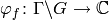 . The
correspondence is very simple. Given a weight modular form , define
. The
correspondence is very simple. Given a weight modular form , define
(6)
We claim  is left -invariant and satisfies the
desired -symmetry on the right.
Indeed, since
is left -invariant and satisfies the
desired -symmetry on the right.
Indeed, since  satisfies the
cocycle property
satisfies the
cocycle property

we have

Moreover, any
stabilizes . Hence

From (5) we have
 , and thus
 .
.
Hence in (6) the weight and the automorphy factor
“untwist” the -action to make
left -invariant. The upshot is that we can study modular forms by
studying the spaces of functions that arise through the construction
(6).
Of course, not every  will arise as for some
  : after
all, is holomorphic and satisfies rather stringent growth
conditions. Pinning down all the requirements is somewhat technical
and is (mostly) done in the sequel.
: after
all, is holomorphic and satisfies rather stringent growth
conditions. Pinning down all the requirements is somewhat technical
and is (mostly) done in the sequel.
A.2.3
Before we define automorphic forms, we need to find the correct
generalizations of our groups  and .
The correct setup is rather technical, but this really reflects the
power of the general theory, which handles so many different
situations (e.g., Maass forms, Hilbert modular forms, Siegel
modular forms, etc.).
and .
The correct setup is rather technical, but this really reflects the
power of the general theory, which handles so many different
situations (e.g., Maass forms, Hilbert modular forms, Siegel
modular forms, etc.).
Let be a connected Lie group, and let  be a maximal
compact subgroup. We assume that is the set of real points of a
connected semisimple algebraic group
be a maximal
compact subgroup. We assume that is the set of real points of a
connected semisimple algebraic group  defined over . These
conditions mean the following [PR84, Section 2.1.1]:
defined over . These
conditions mean the following [PR84, Section 2.1.1]:
The group
has the structure of an affine algebraic variety given by an ideal
 in the ring
 ![R = \C [x_{ij}, D^{-1} ]](_images/math/e52bd8a4069638dd56192202a2aa8d74cdf13c0a.png) , where the variables
, where the variables
 should be interpreted as the entries of
an “indeterminate matrix,” and
should be interpreted as the entries of
an “indeterminate matrix,” and  is the polynomial
 . Both the group multiplication
  and inversion
  are required to be morphisms of
algebraic varieties.
are required to be morphisms of
algebraic varieties.The ring
 is the coordinate ring of the algebraic group
  .
Hence this condition means that can be essentially viewed as a
subgroup of
.
Hence this condition means that can be essentially viewed as a
subgroup of  defined by polynomial equations in the
matrix entries of the latter.
defined by polynomial equations in the
matrix entries of the latter.Defined over
means that is generated by
polynomials with rational coefficients.Connected means that
is connected as an algebraic variety.Set of real points means that
is the set of real
solutions to the equations determined by . We write  .
.Semisimple means that the maximal connected solvable normal subgroup of
is trivial.
Example A.1
The most important example for our purposes is
the split form of  . For this choice we have

Example A.2
Let  be a number field. Then there is a -group such
that
be a number field. Then there is a -group such
that  . The group is constructed as
 , where
  denotes the
restriction of scalars from
denotes the
restriction of scalars from  to
[PR84, Section 2.1.2]. For example, if is totally real, the
group
to
[PR84, Section 2.1.2]. For example, if is totally real, the
group  appears when one studies Hilbert modular
forms.
appears when one studies Hilbert modular
forms.
Let  be the signature of the field , so that
  . Then
  and
and  .
.
Example A.3
Another important example is the split symplectic group
 . This is the group that arises when one studies Siegel
modular forms. The group of real points
. This is the group that arises when one studies Siegel
modular forms. The group of real points  is the
subgroup of
is the
subgroup of  preserving a fixed nondegenerate
alternating bilinear form on
preserving a fixed nondegenerate
alternating bilinear form on  . We have
  .
.
A.2.4
To generalize , we need the notion of an
arithmetic group. This is a discrete subgroup of the
group of rational points  that is commensurable with the set
of integral points
that is commensurable with the set
of integral points  . Here commensurable simply means that
 is a finite index subgroup of both and
; in particular itself is an arithmetic group.
is a finite index subgroup of both and
; in particular itself is an arithmetic group.
Example A.4
For the split form of we have  . A trivial way to obtain other
arithmetic groups is by conjugation: if
. A trivial way to obtain other
arithmetic groups is by conjugation: if  , then
 is also arithmetic.
A more interesting collection of examples is given by the congruence
subgroups. The principal congruence subgroup  is
the group of matrices congruent to the identity modulo for some
fixed integer
is
the group of matrices congruent to the identity modulo for some
fixed integer  . A congruence subgroup is a group
containing for some .
. A congruence subgroup is a group
containing for some .
In higher dimensions there are many candidates to generalize the Hecke
subgroup . For example, one can take the
subgroup of  that is upper-triangular mod . From
a computational perspective, this choice is not so good since its
index in is large. A better choice, and the one that
usually appears in the literature, is to define to be
the subgroup of with bottom row congruent to
that is upper-triangular mod . From
a computational perspective, this choice is not so good since its
index in is large. A better choice, and the one that
usually appears in the literature, is to define to be
the subgroup of with bottom row congruent to  .
.
A.2.5
We are almost ready to define automorphic forms. Let  be the Lie
algebra of , and let
be the Lie
algebra of , and let  be its universal enveloping algebra
over
be its universal enveloping algebra
over  . Geometrically, is just the tangent space at the
identity of the smooth manifold . The algebra is a
certain complex associative algebra canonically built from . The
usual definition would lead us a bit far afield, so we will settle for an
equivalent characterization: can be realized as a certain
subalgebra of the ring of differential operators on
. Geometrically, is just the tangent space at the
identity of the smooth manifold . The algebra is a
certain complex associative algebra canonically built from . The
usual definition would lead us a bit far afield, so we will settle for an
equivalent characterization: can be realized as a certain
subalgebra of the ring of differential operators on  ,
the space of smooth functions on .
,
the space of smooth functions on .
In particular, acts on by left translations: given  and
and  , we define
Then can be identified with the ring of all differential
operators on that are invariant under left
translation. For our purposes the most important part of is
its center  . In
terms of differential operators, consists of those operators
that are also invariant under right translation:
. In
terms of differential operators, consists of those operators
that are also invariant under right translation:
Definition A.5
An automorphic form on with
respect to is a function  satisfying
- for all ,
- the right translates
 span a finite-dimensional
space
span a finite-dimensional
space  of functions,
 - there exists an ideal
 of finite codimension
such that
of finite codimension
such that  annihilates , and
 - satisfies a certain growth condition that we do not
wish to make precise. (In the literature, is said to be
slowly increasing.)
For fixed and , we denote by  the
space of all functions
satisfying the above four conditions. It is a basic theorem, due to
Harish-Chandra [HC68], that is
finite-dimensional.
the
space of all functions
satisfying the above four conditions. It is a basic theorem, due to
Harish-Chandra [HC68], that is
finite-dimensional.
Example A.6
We can identify the cuspidal modular forms in the language
of Definition Definition A.5. Given a modular form , let
 be the function from
(6). Then the map
be the function from
(6). Then the map  identifies
with the subspace
identifies
with the subspace  of functions satisfying
- for all
 ,
,  for all
  ,
, , where
  is the Laplace–Beltrami–Casimir operator and
- is slowly increasing, and
- is cuspidal.
The first four conditions parallel Definition A.5. Item (1) is the
-invariance. Item (2) implies that the right translates of
by  lie in a fixed finite-dimensional
representation of . Item (3) is how holomorphicity appears,
namely that is killed by a certain differential operator.
Finally, item (4) is the usual growth condition.
lie in a fixed finite-dimensional
representation of . Item (3) is how holomorphicity appears,
namely that is killed by a certain differential operator.
Finally, item (4) is the usual growth condition.
The only condition missing from the general
definition is (5), which is an extra constraint placed on to
ensure that it comes from a cusp form. This condition can be
expressed by the vanishing of certain integrals (“constant terms”);
for details we refer to [Bum97, Gel75].
Example A.7
Another important example appears when we set  in (2) in Example
Example A.6 and relax (3) by requiring only that
in (2) in Example
Example A.6 and relax (3) by requiring only that  for some nonzero
  . Such
automorphic forms cannot possibly arise from modular forms, since
there are no nontrivial cusp forms of weight 0. However, there are
plenty of solutions to these conditions: they correspond to
real-analytic cuspidal modular forms of weight 0 and
are known as Maass forms. Traditionally one writes
. Such
automorphic forms cannot possibly arise from modular forms, since
there are no nontrivial cusp forms of weight 0. However, there are
plenty of solutions to these conditions: they correspond to
real-analytic cuspidal modular forms of weight 0 and
are known as Maass forms. Traditionally one writes  . The positivity of
  implies that
  or is purely imaginary.
Maass forms are highly elusive objects. Selberg proved that there are
infinitely many linearly independent Maass forms of full level
(i.e., on ), but to this date no explicit construction of
a single one is known. (Selberg’s argument is indirect and relies on
the trace formula; for an exposition see [Sar03].) For higher
levels some explicit examples can be constructed using theta series
attached to indefinite quadratic forms [Vig77]. Numerically
Maass forms have been well studied; see for example [FL].
In general the arithmetic nature of the eigenvalues
 that correspond to Maass forms is unknown, although a famous
conjecture of Selberg states that for congruence subgroups they
satisfy the inequality
that correspond to Maass forms is unknown, although a famous
conjecture of Selberg states that for congruence subgroups they
satisfy the inequality  (in other words, only purely
imaginary
(in other words, only purely
imaginary  appear above). The truth of this
conjecture would have far-reaching consequences, from analytic number
theory to graph theory [Lub94].
appear above). The truth of this
conjecture would have far-reaching consequences, from analytic number
theory to graph theory [Lub94].
A.2.6
As Example A.6 indicates, there is a notion of cuspidal automorphic form. The exact definition is too technical to state here, but it involves an appropriate generalization of the notion of constant term familiar from modular forms.
There are also Eisenstein series
[Lan66, Art79]. Again the complete definition is technical; we only
mention that there are different types of Eisenstein series
corresponding to certain subgroups of . The Eisenstein series that
are easiest to understand are those built from cusp forms on lower
rank groups. Very explicit formulas for Eisenstein series on
 can be seen in [Bum84]. For a down-to-earth
exposition of some of the Eisenstein series on , we refer to
[Gol05].
can be seen in [Bum84]. For a down-to-earth
exposition of some of the Eisenstein series on , we refer to
[Gol05].
The decomposition of  into cusp forms and
Eisenstein series also generalizes to a general group , although
the statement is much more complicated. The result is a theorem of
Langlands [Lan76] known as the
spectral decomposition of
into cusp forms and
Eisenstein series also generalizes to a general group , although
the statement is much more complicated. The result is a theorem of
Langlands [Lan76] known as the
spectral decomposition of  .
A thorough recent presentation of
this can be found in [MW94].
.
A thorough recent presentation of
this can be found in [MW94].
A.2.7
Let  be the space of all automorphic forms,
where and range over all possibilities. The space
be the space of all automorphic forms,
where and range over all possibilities. The space  is
huge, and the arithmetic significance of much of it is unknown. This
is already apparent for . The automorphic forms
directly connected with arithmetic are the holomorphic modular forms,
not the Maass forms [2] . Thus the question
arises: which automorphic forms in are the most natural
generalization of the modular forms?
is
huge, and the arithmetic significance of much of it is unknown. This
is already apparent for . The automorphic forms
directly connected with arithmetic are the holomorphic modular forms,
not the Maass forms [2] . Thus the question
arises: which automorphic forms in are the most natural
generalization of the modular forms?
One answer is provided by the isomorphisms (1),
(3), (4). These show that modular forms
appear naturally in the cohomology of modular curves. Hence a
reasonable approach is to generalize the left of (1),
(3), (4), and to study the resulting
cohomology groups. This is the approach we will take. One drawback
is that it is not obvious that our generalization has anything to do
with automorphic forms, but we will see eventually that it certainly
does. So we begin by looking for an appropriate generalization of the
modular curve .
Let and be as in Section A.2.3, and let  be the quotient
. This is a global Riemannian symmetric space [Hel01]. One can prove
that is contractible. Any arithmetic group
be the quotient
. This is a global Riemannian symmetric space [Hel01]. One can prove
that is contractible. Any arithmetic group  acts
on properly discontinuously. In particular, if is
torsion-free, then the quotient
acts
on properly discontinuously. In particular, if is
torsion-free, then the quotient  is a smooth
manifold.
is a smooth
manifold.
Unlike the modular curves, will not have a
complex structure in general [3]; nevertheless,
is a very nice space. In particular, if
is torsion-free, it is an Eilenberg–Mac Lane space for
, otherwise known as a  . This means that the
only nontrivial homotopy group of is its
fundamental group, which is isomorphic to , and that the
universal cover of is contractible. Hence
is in some sense a “topological
incarnation” [4] of .
. This means that the
only nontrivial homotopy group of is its
fundamental group, which is isomorphic to , and that the
universal cover of is contractible. Hence
is in some sense a “topological
incarnation” [4] of .
This leads us to the notion of the group cohomology  of with trivial complex coefficients. In the
early days of algebraic topology, this was defined to be the complex
cohomology of an Eilenberg–Mac~Lane space for
[Bro94, Introduction, I.4]:
of with trivial complex coefficients. In the
early days of algebraic topology, this was defined to be the complex
cohomology of an Eilenberg–Mac~Lane space for
[Bro94, Introduction, I.4]:
(7)
Today there are purely algebraic approaches to  [Bro94, III.1], but for our purposes (7) is
exactly what we need. In fact, the group cohomology
[Bro94, III.1], but for our purposes (7) is
exactly what we need. In fact, the group cohomology  can be identified with the cohomology of the quotient
  even if has torsion, since we are working with
complex coefficients. The cohomology groups
even if has torsion, since we are working with
complex coefficients. The cohomology groups  ,
where is an arithmetic group, are our proposed generalization
for the weight 2 modular forms.
,
where is an arithmetic group, are our proposed generalization
for the weight 2 modular forms.
What about higher weights? For this we must replace the trivial
coefficient module with local systems, just as we did in
(3). For our purposes it is enough to let  be a
rational finite-dimensional representation of over the complex
numbers. Any such gives a representation of
be a
rational finite-dimensional representation of over the complex
numbers. Any such gives a representation of  and thus induces a local system
  on . As before, the group cohomology
  is the cohomology
  . In (3) we took
  , the
, the
 symmetric power of the standard representation. For a general
group there are many kinds of representations to consider. In any
case, we contend that the cohomology spaces
symmetric power of the standard representation. For a general
group there are many kinds of representations to consider. In any
case, we contend that the cohomology spaces

are a good generalization of the spaces of modular forms.
A.2.8
It is certainly not obvious that the cohomology groups
 have anything to do with automorphic forms, although
the isomorphisms (1), (3), (4) look
promising.
have anything to do with automorphic forms, although
the isomorphisms (1), (3), (4) look
promising.
The connection is provided by a deep theorem of Franke [Fra98], which asserts that
the cohomology groups
 can be directly
computed in terms of certain automorphic forms (the automorphic forms
of “cohomological type,” also known as those with “nonvanishing
can be directly
computed in terms of certain automorphic forms (the automorphic forms
of “cohomological type,” also known as those with “nonvanishing
 cohomology” [VZ84]); and
there is a direct sum decomposition
(8)
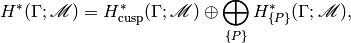
where the sum is taken over the set of classes of associate proper
-parabolic subgroups of .
The precise version of statement (?) is known in the literature
as the Borel conjecture. Statement (8) parallels
Langlands’s spectral decomposition of .
Example A.8
For , the decomposition
(8) is exactly (4). The cuspforms
 correspond to the summand
 . There is one class of proper
-parabolic subgroups in , represented by the Borel subgroup
of upper-triangular matrices. Hence only one term appears in big
direct sum on the right of (8), which is the
Eisenstein term
. There is one class of proper
-parabolic subgroups in , represented by the Borel subgroup
of upper-triangular matrices. Hence only one term appears in big
direct sum on the right of (8), which is the
Eisenstein term
 .
.
The summand  of
(8) is called the cuspidal cohomology; this
is the subspace of classes represented by cuspidal automorphic forms.
The remaining summands constitute the Eisenstein cohomology of
[Har91]. In particular the summand indexed by
of
(8) is called the cuspidal cohomology; this
is the subspace of classes represented by cuspidal automorphic forms.
The remaining summands constitute the Eisenstein cohomology of
[Har91]. In particular the summand indexed by  is
constructed using Eisenstein series attached to certain cuspidal
automorphic forms on lower rank groups. Hence
is
constructed using Eisenstein series attached to certain cuspidal
automorphic forms on lower rank groups. Hence  is in some sense the most important part of the
cohomology: all the rest can be built systematically from cuspidal
cohomology on lower rank groups [5]. This leads us to our
basic computational problem:
is in some sense the most important part of the
cohomology: all the rest can be built systematically from cuspidal
cohomology on lower rank groups [5]. This leads us to our
basic computational problem:
Problem A.9
Develop tools to compute explicitly the cohomology spaces
 and to identify the cuspidal
subspace
and to identify the cuspidal
subspace  .
.
A.3 Combinatorial Models for Group Cohomology
A.3.1
In this section, we restrict attention to  and
, a congruence subgroup of . By the previous
section, we can study the group cohomology by
studying the cohomology
and
, a congruence subgroup of . By the previous
section, we can study the group cohomology by
studying the cohomology  . The latter spaces can be studied using standard
topological techniques, such as taking the cohomology of complexes
associated to cellular decompositions of . For
. The latter spaces can be studied using standard
topological techniques, such as taking the cohomology of complexes
associated to cellular decompositions of . For
 , one can construct such decompositions using a
version of explicit reduction theory of real positive-definite
quadratic forms due to Voronoi [Vor08]. The goal of this section is
to explain how this is done. We also discuss how the cohomology can
be explicitly studied for congruence subgroups of
, one can construct such decompositions using a
version of explicit reduction theory of real positive-definite
quadratic forms due to Voronoi [Vor08]. The goal of this section is
to explain how this is done. We also discuss how the cohomology can
be explicitly studied for congruence subgroups of  .
.
A.3.2
Let  be the
  -vector space of all symmetric
  matrices, and let
  be the subset of positive-definite
matrices. The space
be the subset of positive-definite
matrices. The space  can be identified with the space of all real
positive-definite quadratic forms in variables: in coordinates, if
can be identified with the space of all real
positive-definite quadratic forms in variables: in coordinates, if
 (column vector), then the matrix
 induces the
quadratic form
induces the
quadratic form

and it is well known that any positive-definite quadratic form arises
in this way. The space is a cone, in that it is preserved by
homotheties: if  , then
  for all
  . It is also convex: if
  , then
  for
for ![t\in [0,1]](_images/math/f59b2675d4485df7a52a77eb0d7ea513eae7e947.png) . Let be the quotient of by
homotheties.
. Let be the quotient of by
homotheties.
Example A.10
The case  is illustrative. We can take
coordinates on
is illustrative. We can take
coordinates on  by representing any matrix in as
The subset of singular matrices  is a quadric
cone in dividing the complement
is a quadric
cone in dividing the complement  into three
connected components. The component containing the identity matrix is
the cone of positive-definite matrices. The quotient can be
identified with an open
into three
connected components. The component containing the identity matrix is
the cone of positive-definite matrices. The quotient can be
identified with an open  -disk.
The group acts on on the left by
This action commutes with that of the homotheties and thus
descends to a -action on . One can show that acts transitively
on and that the stabilizer of the image of the identity matrix is
 . Hence we may identify with our symmetric space
  . We will do this in the sequel, using the
notation when we want to emphasize the coordinates coming from the
linear structure of and using the notation for the
quotient .
. We will do this in the sequel, using the
notation when we want to emphasize the coordinates coming from the
linear structure of and using the notation for the
quotient .
We can make the identification  more explicit. If
  , then the map
(9)
takes  to a symmetric positive-definite matrix. Any coset
  is
taken to the same matrix since
is
taken to the same matrix since  . Thus (9)
identifies with a subset
. Thus (9)
identifies with a subset  of , namely those
positive-definite symmetric matrices with determinant
of , namely those
positive-definite symmetric matrices with determinant  . It is
easy to see that maps diffeomorphically onto .
. It is
easy to see that maps diffeomorphically onto .
The inverse map  is more complicated. Given a
determinant positive-definite symmetric matrix
is more complicated. Given a
determinant positive-definite symmetric matrix  , one must find
 such that
  . Such a representation
always exists, with determined uniquely up to right multiplication
by an element of . In computational linear algebra, such a can
be constructed through Cholesky decomposition of .
. Such a representation
always exists, with determined uniquely up to right multiplication
by an element of . In computational linear algebra, such a can
be constructed through Cholesky decomposition of .
The group  acts on via the -action and does so
properly discontinuously. This is the “unimodular change of
variables” action on quadratic forms [Ser73, V.1.1].
Under our identification of with , this is the usual action of
by left translation from Section A.2.7.
acts on via the -action and does so
properly discontinuously. This is the “unimodular change of
variables” action on quadratic forms [Ser73, V.1.1].
Under our identification of with , this is the usual action of
by left translation from Section A.2.7.
A.3.3
Now consider the group cohomology  . The identification
  shows that the dimension of is
  . Hence
  vanishes if
  . Since
  grows quadratically in , there are many potentially interesting
cohomology groups to study.
grows quadratically in , there are many potentially interesting
cohomology groups to study.
However, it turns out that there is some additional vanishing of the
cohomology for deeper (topological) reasons. For , this is easy
to see. The quotient is homeomorphic to a
topological surface with punctures, corresponding to the cusps of
. Any such surface  can be retracted onto a finite graph
simply by “stretching” along its punctures. Thus
can be retracted onto a finite graph
simply by “stretching” along its punctures. Thus  , even though
  .
.
For  , a theorem of Borel–Serre implies
that
, a theorem of Borel–Serre implies
that  vanishes if
  [BS73, Theorem 11.4.4]. The number
  is
called the virtual cohomological dimension of and is
denoted
is
called the virtual cohomological dimension of and is
denoted  . Thus we only need to consider cohomology in
degrees
. Thus we only need to consider cohomology in
degrees  .
.
Moreover we know from Section A.2.8 that the most interesting part
of the cohomology is the cuspidal cohomology. In what degrees can it
live? For , there is only one interesting cohomology group
 , and it contains the cuspidal cohomology. For
higher dimensions, the situation is quite different: for most , the
subspace
, and it contains the cuspidal cohomology. For
higher dimensions, the situation is quite different: for most , the
subspace  vanishes! In fact in
the late 1970’s Borel, Wallach, and Zuckerman observed that the cuspidal
cohomology can only live in the cohomological degrees lying in an
interval around
vanishes! In fact in
the late 1970’s Borel, Wallach, and Zuckerman observed that the cuspidal
cohomology can only live in the cohomological degrees lying in an
interval around  of size linear in . An explicit
description of this interval is given in
[Sch86, Proposition 3.5];
one can also look at Table A.1, from which
the precise statement is easy to determine.
of size linear in . An explicit
description of this interval is given in
[Sch86, Proposition 3.5];
one can also look at Table A.1, from which
the precise statement is easy to determine.
Another feature of Table A.1 deserves to be mentioned.
There are exactly two values of , namely  , such that
virtual cohomological dimension equals the upper limit of the cuspidal
range. This will have implications later, when we study the action of
the Hecke operators on the cohomology.
, such that
virtual cohomological dimension equals the upper limit of the cuspidal
range. This will have implications later, when we study the action of
the Hecke operators on the cohomology.
Table A.1
The virtual cohomological dimension and the cuspidal range
for subgroups of  .
.
![\begin{table}[htb]
\begin{center}
\begin{tabular}{c||c|c|c|c|c|c|c|c}
$n$&2&3&4&5&6&7&8&9\cr
\hline
\hline
$\dim X$&2 & 5 & 9 & 14 & 20 & 27 & 35 & 44 \cr
$\vcd \Gamma $ & 1 & 3 & 6 & 10 & 15 & 21 & 28 & 36\cr
top degree of $H^{*}_{\text{cusp}} $& 1 & 3 & 5 & 8 & 11 & 15 & 19& 24 \cr
bottom degree of $H^{*}_{\text{cusp}} $& 1 & 2 & 4 & 6 & 9 & 12 & 16 & 20 \cr
\end{tabular}
\end{center}
\medskip
\caption{}
\end{table}](_images/math/8a126bf6f7186380e2b34aa6772722344ff3072b.png)
A.3.4
Recall that a point in  is said to be primitive if the
greatest common divisor of its coordinates is . In particular, a
primitive point is nonzero. Let
is said to be primitive if the
greatest common divisor of its coordinates is . In particular, a
primitive point is nonzero. Let  be the set of
primitive points. Any
be the set of
primitive points. Any  , written as a column vector,
determines a rank- symmetric matrix
, written as a column vector,
determines a rank- symmetric matrix  in the closure
  via
via  . The Voronoi polyhedron
  is defined
to be the closed convex hull in of the points , as
is defined
to be the closed convex hull in of the points , as  ranges over
  . Note that by construction, acts
on , since preserves the set
. Note that by construction, acts
on , since preserves the set  and
acts linearly on .
and
acts linearly on .
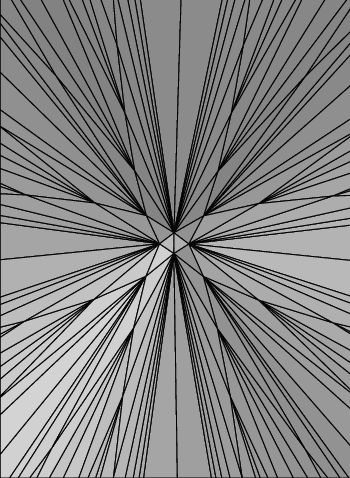
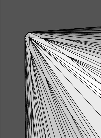
Example A.11
Figure A.1 represents a crude attempt to show what
looks like for . These images were constructed by computing a
large subset of the points and taking the convex hull (we took
all points such that  for some large
integer ). From a distance, the polyhedron looks almost
indistinguishable from the cone ; this is somewhat conveyed by the
right of Figure A.1. Unfortunately is not locally
finite, so we really cannot produce an accurate picture. To get a more
accurate image, the reader should imagine that each vertex meets
infinitely many edges. On the other hand, is not hopelessly
complex: each maximal face is a triangle, as the pictures suggest.
for some large
integer ). From a distance, the polyhedron looks almost
indistinguishable from the cone ; this is somewhat conveyed by the
right of Figure A.1. Unfortunately is not locally
finite, so we really cannot produce an accurate picture. To get a more
accurate image, the reader should imagine that each vertex meets
infinitely many edges. On the other hand, is not hopelessly
complex: each maximal face is a triangle, as the pictures suggest.
Figure A.1
The polyhedron for . In (a) we see from
the origin, in (b) from the side. The small triangle at the right
center of (a) is the facet with vertices
 , where
 is the standard basis of
 . In (b) the
  -axis runs along the top from left to
right, and the
-axis runs along the top from left to
right, and the  -axis runs down the left side. The facet
from (a) is the little triangle at the top left corner of (b).
-axis runs down the left side. The facet
from (a) is the little triangle at the top left corner of (b).
A.3.5
The polyhedron is quite complicated: it has infinitely many
faces and is not locally finite. However, one of Voronoi ‘s great
insights is that is actually not as complicated as it seems.
For any , let  be the minimum value attained by
on and let
be the minimum value attained by
on and let  be the set on which attains
. Note that
be the set on which attains
. Note that  and
and  is finite since is
positive-definite. Then is called perfect if it is
recoverable from the knowledge of the pair
is finite since is
positive-definite. Then is called perfect if it is
recoverable from the knowledge of the pair  . In
other words, given , we can write a system of
linear equations
. In
other words, given , we can write a system of
linear equations
(10)
where  is a symmetric matrix of variables. Then is
perfect if and only if is the unique solution to the system
(10).
is a symmetric matrix of variables. Then is
perfect if and only if is the unique solution to the system
(10).
Example A.12
The quadratic form  is perfect. The smallest
nontrivial value
it attains on is
is perfect. The smallest
nontrivial value
it attains on is  , and it does so on the columns of
and their negatives. Letting  be an undetermined quadratic form and applying the data
  , we are led to the system of linear equations

From this we recover  .
.
Example A.13
The quadratic form  is not perfect. Again the
smallest nontrivial value of
is not perfect. Again the
smallest nontrivial value of  on is
on is  , attained on the
columns of
, attained on the
columns of
and their negatives. But every member of the one-parameter family of quadratic forms
(11)
has the same
set of minimal vectors, and so cannot be recovered from the
knowledge of  .
.
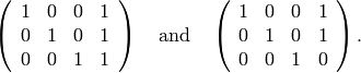
Example A.14
Example A.12 generalizes to all . Define
(12)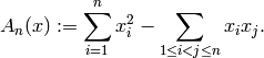
Then  is perfect for all . We have
  , and
, and  consists of all points of the form

where  is the standard basis of
  . This quadratic
form is closely related to the root lattice
[FH91], which explains its name. It is one of two
infinite families of perfect forms studied by Voronoi (the other is
related to the
. This quadratic
form is closely related to the root lattice
[FH91], which explains its name. It is one of two
infinite families of perfect forms studied by Voronoi (the other is
related to the  root lattice).
We can now summarize Voronoi ‘s main results:
- There are finitely many equivalence classes of perfect forms
modulo the action of . Voronoi even gave an explicit
algorithm to determine all the perfect forms of a given dimension.
- The facets of , in other words the
codimension faces, are in bijection with the rank perfect
quadratic forms. Under this correspondence the minimal vectors
 determine a facet
  by taking the convex hull in
of the finite point set
by taking the convex hull in
of the finite point set  . Hence there are
finitely many faces of modulo and thus finitely
many modulo any finite index subgroup .
. Hence there are
finitely many faces of modulo and thus finitely
many modulo any finite index subgroup . - Let
 be the set of cones over the faces of . Then
is a fan, which means (i) if
be the set of cones over the faces of . Then
is a fan, which means (i) if  , then any face of
 is also in ; and (ii) if
  , then
 is a common face of each [6]. The fan provides a
reduction theory for in the following sense: any point is
contained in a unique
is a common face of each [6]. The fan provides a
reduction theory for in the following sense: any point is
contained in a unique  , and the set
  is
finite. Voronoialso gave an explicit algorithm to determine
is
finite. Voronoialso gave an explicit algorithm to determine  given , the Voronoi reduction algorithm.
The number  of equivalence classes of perfect forms modulo the
action of
of equivalence classes of perfect forms modulo the
action of  grows rapidly with
(Table A.2); the complete classification is known
only for
grows rapidly with
(Table A.2); the complete classification is known
only for  . For a list of perfect forms up to
  , see
[CS88]. For a recent comprehensive treatment of perfect forms,
with many historical remarks, see
[Mar03].
, see
[CS88]. For a recent comprehensive treatment of perfect forms,
with many historical remarks, see
[Mar03].
A.3.6
Our goal now is to describe how the Voronoi
fan can be used to compute the cohomology . The idea is to use the cones in to chop the quotient
into pieces.
For any , let  be the open cone
obtained by taking the complement in of its proper faces.
Then after taking the quotient by homotheties, the cones
be the open cone
obtained by taking the complement in of its proper faces.
Then after taking the quotient by homotheties, the cones  pass to locally closed subsets of .
Let
pass to locally closed subsets of .
Let  be the set of these images.
Any  is a topological cell, i.e., it is homeomorphic to
an open ball, since
is a topological cell, i.e., it is homeomorphic to
an open ball, since  is homeomorphic to a face of . Because
comes from the fan , the cells in have good incidence
properties: the closure in of any can be written as a
finite disjoint union of elements of . Moreover, is
locally finite: by taking quotients of all the
is homeomorphic to a face of . Because
comes from the fan , the cells in have good incidence
properties: the closure in of any can be written as a
finite disjoint union of elements of . Moreover, is
locally finite: by taking quotients of all the  meeting , we have eliminated the open cones lying in , and
it is these cones that are responsible for the failure of local
finiteness of . We summarize these properties by saying that
gives a cellular decomposition of . Clearly
meeting , we have eliminated the open cones lying in , and
it is these cones that are responsible for the failure of local
finiteness of . We summarize these properties by saying that
gives a cellular decomposition of . Clearly  acts on , since is constructed using the fan .
Thus we obtain a cellular decomposition [7] of
acts on , since is constructed using the fan .
Thus we obtain a cellular decomposition [7] of  for
any torsion-free . We call the Voronoi decomposition of .
for
any torsion-free . We call the Voronoi decomposition of .
Some care must be taken in using these cells to perform topological computations. The problem is that even though the individual pieces are homeomorphic to balls and are glued together nicely, the boundaries of the closures of the pieces are not homeomorphic to spheres in general. (If they were, then the Voronoi decomposition would give rise to a regular cell complex [CF67], which can be used as a substitute for a simplicial or CW complex in homology computations.) Nevertheless, there is a way to remedy this.
Recall that a subspace of a topological space  is a
strong deformation retract if there is a continuous map
is a
strong deformation retract if there is a continuous map
![f\colon B\times [0,1]\rightarrow B](_images/math/344b4b2eaf548613556ee0591f6fdbb9d67b5308.png) such that
such that  ,
,  , and
, and  for all
  . For such pairs
 we have
  . One can show that there
is a strong deformation retraction from to itself equivariant
under the actions of both
. One can show that there
is a strong deformation retraction from to itself equivariant
under the actions of both  and the homotheties and that
the image of the retraction modulo homotheties, denoted
and the homotheties and that
the image of the retraction modulo homotheties, denoted  , is
naturally a locally finite regular cell complex of dimension
, is
naturally a locally finite regular cell complex of dimension  .
Moreover, the cells in are in bijective, inclusion-reversing
correspondence with the cells in . In particular, if a cell in
has codimension
.
Moreover, the cells in are in bijective, inclusion-reversing
correspondence with the cells in . In particular, if a cell in
has codimension  , the corresponding cell in has
dimension . Thus, for example, the vertices of modulo
are in bijection with the top-dimensional cells in
, which are in bijection with equivalence classes of perfect
forms.
, the corresponding cell in has
dimension . Thus, for example, the vertices of modulo
are in bijection with the top-dimensional cells in
, which are in bijection with equivalence classes of perfect
forms.
In the literature is called the well-rounded retract. The
subspace  has a beautiful geometric
interpretation. The quotient
has a beautiful geometric
interpretation. The quotient

can be interpreted as the moduli space of lattices in  modulo
the equivalence relation of rotation and positive scaling
(cf. [AG00]; for one can also see
[Ser73, VII, Proposition 3]).
Then corresponds to those lattices whose
shortest nonzero vectors span . This is the origin of the
name: the shortest vectors of such a lattice are “more round” than
those of a generic lattice.
modulo
the equivalence relation of rotation and positive scaling
(cf. [AG00]; for one can also see
[Ser73, VII, Proposition 3]).
Then corresponds to those lattices whose
shortest nonzero vectors span . This is the origin of the
name: the shortest vectors of such a lattice are “more round” than
those of a generic lattice.
The space was known classically for and was constructed for
 by Lannes and Soul’e, although Soul’e only published the
case
by Lannes and Soul’e, although Soul’e only published the
case  [Sou75]. The construction for all appears in work
of Ash [Ash80, Ash84], who also generalized to a much
larger class of groups. Explicit computations of the cell structure
of have only been performed up to
[Sou75]. The construction for all appears in work
of Ash [Ash80, Ash84], who also generalized to a much
larger class of groups. Explicit computations of the cell structure
of have only been performed up to  [EVGS02]. Certainly
computing explicitly for
[EVGS02]. Certainly
computing explicitly for  seems very difficult, as
Table A.2 indicates.
seems very difficult, as
Table A.2 indicates.
Example A.15
Figure A.2 illustrates and for . As in
Example A.11, the polyhedron is 3-dimensional, and
so the Voronoi fan has cones of dimensions  . The
-cones of , which correspond to the vertices of , pass to
infinitely many points on the boundary
. The
-cones of , which correspond to the vertices of , pass to
infinitely many points on the boundary  . The
. The  -cones become triangles in
  with
vertices on
with
vertices on  . In fact, the identifications
 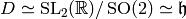 realize as the Klein model for the
hyperbolic plane, in which geodesics are represented by Euclidean line
segments. Hence, the images of the -cones of are none other
than the usual cusps of , and the triangles are the
realize as the Klein model for the
hyperbolic plane, in which geodesics are represented by Euclidean line
segments. Hence, the images of the -cones of are none other
than the usual cusps of , and the triangles are the  -translates of the ideal triangle with vertices
  . These triangles form a tessellation of sometimes known as
the Farey tessellation. The edges of the Voronoi are the -translates of the ideal geodesic between
. These triangles form a tessellation of sometimes known as
the Farey tessellation. The edges of the Voronoi are the -translates of the ideal geodesic between  and
and  .
After adjoining cusps and passing to the quotient , these
edges become the supports of the Manin symbols from Section Manin Symbols
(cf. Figure 3.2). This example also shows how the
Voronoi decomposition fails to be a regular cell complex: the
boundaries of the closures of the triangles in do not contain the
vertices and thus are not homeomorphic to circles.
.
After adjoining cusps and passing to the quotient , these
edges become the supports of the Manin symbols from Section Manin Symbols
(cf. Figure 3.2). This example also shows how the
Voronoi decomposition fails to be a regular cell complex: the
boundaries of the closures of the triangles in do not contain the
vertices and thus are not homeomorphic to circles.
The virtual cohomological dimension of is 1. Hence the
well-rounded retract is a graph (Figure A.2 and
Figure A.3). Note that is not a manifold. The vertices
of are in bijection with the Farey triangles—each vertex lies at
the center of the corresponding triangle—and the edges are in
bijection with the Manin symbols. Under the map  ,
the graph becomes the familiar “
,
the graph becomes the familiar “ -tree” embedded in
, with vertices at the order 3 elliptic points (Figure A.3).
-tree” embedded in
, with vertices at the order 3 elliptic points (Figure A.3).
Figure A.2
The Voronoi decomposition and the retract in
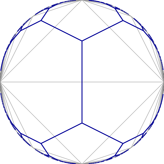
Figure A.3
The Voronoi decomposition and the retract in .
A.3.7
We now discuss the example in some detail. This
example gives a good feeling for how the general situation compares to
the case .
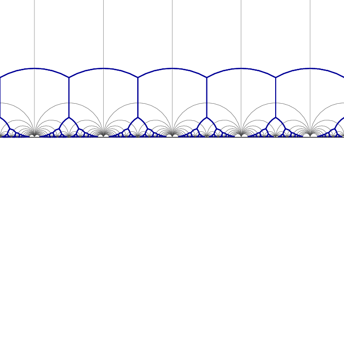
We begin with the Voronoi fan . The cone is 6-dimensional, and
the quotient is 5-dimensional. There is one equivalence class of
perfect forms modulo the action of  , represented by the
form (12). Hence there are 12 minimal vectors; six are the
columns of the matrix
, represented by the
form (12). Hence there are 12 minimal vectors; six are the
columns of the matrix
(13)
and the remaining six are the negatives of these. This implies that
the cone corresponding to this form is 6-dimensional and
simplicial. The latter implies that the faces of are the
cones generated by 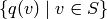 , where ranges over all
subsets of (13). To get the full structure of the fan,
one must determine the orbits of faces, as well as
which faces lie in the boundary
, where ranges over all
subsets of (13). To get the full structure of the fan,
one must determine the orbits of faces, as well as
which faces lie in the boundary  . After some pleasant computation, one finds:
There is one equivalence class modulo
for each of the
6-, 5-, 2-, and 1-dimensional cones.There are two equivalence classes of the 4-dimensional cones, represented by the sets of minimal vectors
There are two equivalence classes of the 3-dimensional cones, represented by the sets of minimal vectors
The second type of 3-cone lies in
 and thus does
not determine a cell in .
and thus does
not determine a cell in .The 2- and 1-dimensional cones lie entirely in
and do not determine cells in .
After passing from to , the cones of dimension determine
cells of dimension  .
Therefore, modulo the action of there are five types of
cells in the Voronoi decomposition , with dimensions from
.
Therefore, modulo the action of there are five types of
cells in the Voronoi decomposition , with dimensions from  to .
We denote these cell types by
to .
We denote these cell types by  ,
,  ,
,  ,
,  ,
and
,
and  . Here corresponds to the first type of 4-cone in item
(?) above, and to the second. For a beautiful way
to index the cells of using configurations in projective spaces,
see [McC91].
. Here corresponds to the first type of 4-cone in item
(?) above, and to the second. For a beautiful way
to index the cells of using configurations in projective spaces,
see [McC91].
The virtual cohomological dimension of is 3, which
means that the retract is a 3-dimensional cell complex. The
closures of the top-dimensional cells in , which are in bijection
with the Voronoi cells of type , are homeomorphic to solid cubes
truncated along two pairs of opposite corners
(Figure A.4). To compute this, one must see how many Voronoi cells
of a given type contain a fixed cell of type (since the
inclusions of cells in are the opposite of those in ).
A table of the incidence relations between the cells of and
is given in Table A.3. To interpret the table, let  be the integer in row and column
  .
.
- If
 is below the diagonal, then the boundary of a cell
of type contains cells of type .
is below the diagonal, then the boundary of a cell
of type contains cells of type . - If is above the diagonal, then a cell of type
appears in the boundary of cells of type .
For instance, the entry  in row and column means
that a Voronoi cell of type meets the boundaries of cells
of type . This is the same as the number of vertices in the
Soul’e cube (Figure A.4).
Investigation of the table shows that the triangular
(respectively, hexagonal) faces of the Soul’e cube correspond to the
Voronoi cells of type (resp., ).
in row and column means
that a Voronoi cell of type meets the boundaries of cells
of type . This is the same as the number of vertices in the
Soul’e cube (Figure A.4).
Investigation of the table shows that the triangular
(respectively, hexagonal) faces of the Soul’e cube correspond to the
Voronoi cells of type (resp., ).
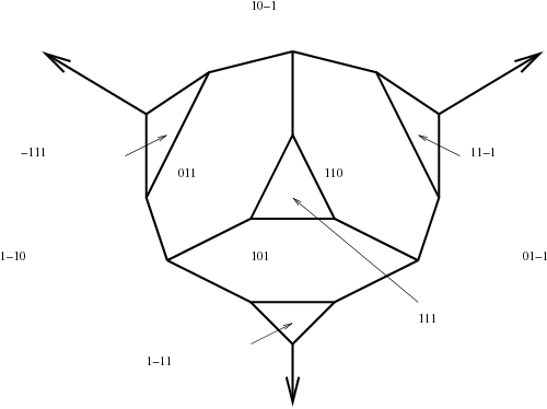
Figure A.5 shows a Schlegel diagram for the Soul’e
cube. One vertex is at infinity; this is indicated by the arrows on
three of the edges. This Soul’e cube is dual to the Voronoi cell of
type with minimal vectors given by the columns of the identity
matrix. The labels on the -faces are additional minimal vectors
that show which Voronoi cells contain . For example, the central
triangle labelled with  is dual to the Voronoi cell of type
with minimal vectors given by those of together with
. Cells of type containing in their closure
correspond to the edges of the figure; the minimal vectors for a given
edge are those of together with the two vectors on the -faces
containing the edge. Similarly, one can read off the minimial vectors
of the top-dimensional Voronoi cells containing , which correspond to
the vertices of Figure A.5.
is dual to the Voronoi cell of type
with minimal vectors given by those of together with
. Cells of type containing in their closure
correspond to the edges of the figure; the minimal vectors for a given
edge are those of together with the two vectors on the -faces
containing the edge. Similarly, one can read off the minimial vectors
of the top-dimensional Voronoi cells containing , which correspond to
the vertices of Figure A.5.
Table A.3
Incidence relations in the Voronoi decomposition and the retract
for .
![\begin{table}[htb]
\begin{center}
\begin{tabular*}{0.75\textwidth}{@{\extracolsep{\fill}}c||c|c|c|c|c}
&$c_{5}$& $c_{4}$& $c_{3a}$& $c_{3b}$& $c_{2}$\\
\hline
\hline
$c_{5}$& $\bullet$& $2$& $3$& $6$& $16$\\
$c_{4}$& $6$& $\bullet$& $3$& $6$& $24$\\
$c_{3a}$& $3$& $1$& $\bullet$& $\bullet$& $4$\\
$c_{3b}$& $12$& $4$& $\bullet$& $\bullet$& $6$\\
$c_{2}$& $12$& $8$& $4$& $3$& $\bullet$\\
\end{tabular*}
\end{center}
\medskip
\caption{}
\end{table}](_images/math/af5f939c34b08610686e7f2a66b55cba651bc466.png)
Figure A.4
The Soul’e cube
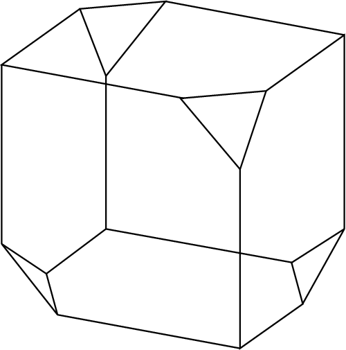
Figure A.5
A Schlegel diagram of a Soul’e cube, showing the minimal
vectors that correspond to the -faces.
A.3.8
Now let  be a prime, and let
  be the Hecke subgroup of matrices with bottom row
congruent to
be the Hecke subgroup of matrices with bottom row
congruent to  (Example A.4). The
virtual cohomological dimension of is , and the cusp
cohomology with constant coefficients can appear in degrees and
. One can show that the cusp cohomology in degree is dual to
that in degree , so for computational purposes it suffices to focus
on degree .
(Example A.4). The
virtual cohomological dimension of is , and the cusp
cohomology with constant coefficients can appear in degrees and
. One can show that the cusp cohomology in degree is dual to
that in degree , so for computational purposes it suffices to focus
on degree .
In terms of , these will be cochains supported on the 3-cells.
Unfortunately we cannot work directly with the quotient  since has torsion: there will be cells taken to
themselves by the -action, and thus the cells of need to
be subdivided to induce the structure of a cell complex on . Thus when has torsion, the “set of -cells
modulo ” unfortunately makes no sense.
since has torsion: there will be cells taken to
themselves by the -action, and thus the cells of need to
be subdivided to induce the structure of a cell complex on . Thus when has torsion, the “set of -cells
modulo ” unfortunately makes no sense.
To circumvent this problem, one can mimic the idea of Manin symbols.
The quotient  is in bijection with the
finite projective plane
is in bijection with the
finite projective plane  , where
  is the
field with elements (cf. Proposition 3.10).
The group acts transitively on the set of all -cells
of ; if we fix one such cell
is the
field with elements (cf. Proposition 3.10).
The group acts transitively on the set of all -cells
of ; if we fix one such cell  , its stabilizer
  is a finite subgroup
of . Hence the set of -cells modulo should
be interpreted as the set of orbits in of the
finite group
is a finite subgroup
of . Hence the set of -cells modulo should
be interpreted as the set of orbits in of the
finite group  . This suggests describing
  in terms of the space
  of complex-valued functions
  . To carry this out, there are two problems:
- How do we explicitly describe in terms of ?
- How can we isolate the cuspidal subspace
 in terms of our description?
Fully describing the solutions to these problems is rather complicated. We content ourselves with presenting the following theorem, which collects together several statements in [AGG84]. This result should be compared to Theorems Theorem 3.13 and Theorem 1.25.
Theorem A.16
We have

where  is the dimension of the space of weight holomorphic
cusp forms on
is the dimension of the space of weight holomorphic
cusp forms on  . Moreover,
the cuspidal cohomology
. Moreover,
the cuspidal cohomology  is isomorphic to the vector space of functions
  satisfying
 ,
, ,
, , and
, and .
.
Unlike subgroups of , cuspidal cohomology is
apparently much rarer for  . The
computations of [AGG84, vGvdKTV97] show that the only prime levels
. The
computations of [AGG84, vGvdKTV97] show that the only prime levels
 with nonvanishing cusp cohomology are
  ,
,  ,
,  ,
,  ,
and
,
and  . In all these examples, the cuspidal subspace is
-dimensional.
. In all these examples, the cuspidal subspace is
-dimensional.
For more details of how to implement such computations, we refer to
[AGG84, vGvdKTV97]. For further details about the additional
complications arising for higher rank groups, in particular subgroups
of  , see [AGM02, Section 3].
A.4 Hecke Operators and Modular Symbols
A.4.1
There is one ingredient missing so far in our discussion of the cohomology of arithmetic groups, namely the Hecke operators.index{Hecke operator} These are an essential tool in the study of modular forms. Indeed, the forms with the most arithmetic significance are the Hecke eigenforms, and the connection with arithmetic is revealed by the Hecke eigenvalues.
In higher rank the situation is similar. There is an algebra of
Hecke operators acting on the cohomology spaces . The eigenvalues of these operators are conjecturally related
to certain representations of the Galois group. Just as in the case
, we need tools to compute the Hecke action.
In this section we discuss this problem. We begin with a general
description of the Hecke operators and how they act on cohomology.
Then we focus on one particular cohomology group, namely the top
degree  , where
  and
has finite index in . This is the setting that
generalizes the modular symbols method from Chapter General Modular Symbols.
We conclude by giving examples of Hecke eigenclasses in the cuspidal
cohomology of .
and
has finite index in . This is the setting that
generalizes the modular symbols method from Chapter General Modular Symbols.
We conclude by giving examples of Hecke eigenclasses in the cuspidal
cohomology of .
A.4.2
Let . The group  has finite index in both and
  . The element determines a diagram
![\xymatrix{&{\Gamma'\backslash X}\ar[dl]_{s}\ar[dr]^{t}&\\
{\Gamma\backslash X}&&{\Gamma\backslash X}}](_images/math/488c85632db35b3e4469a357d35ef892073a2dcb.png)
called a Hecke correspondence. The map is induced by the
inclusion  , while
  is induced by the
inclusion
is induced by the
inclusion  followed by the
diffeomorphism
followed by the
diffeomorphism  given by left multiplication by . Specifically,

The maps and are finite-to-one, since the indices ![[\Gamma
':\Gamma]](_images/math/9b5d54dfe910e64b49f7f9bf681d148e636fffef.png) and
and ![[\Gamma ':g^{-1}\Gamma g]](_images/math/a0662b03bbdcf90475728fea215bc464b9864f9c.png) are finite. This implies
that we obtain maps on cohomology
are finite. This implies
that we obtain maps on cohomology

Here the map  is the usual induced map on cohomology, while the
“wrong-way” map [8]
is the usual induced map on cohomology, while the
“wrong-way” map [8]  is given by summing a class over the finite
fibers of . These maps can be composed to give a map
is given by summing a class over the finite
fibers of . These maps can be composed to give a map

This is called the Hecke operator associated to . There is
an obvious notion of isomorphism of Hecke correspondences. One can
show that up to isomorphism, the correspondence and thus the
Hecke operator  depend only on the double coset
  . One can compose Hecke correspondences, and thus we obtain
an algebra of operators acting on the cohomology, just as in the
classical case.
. One can compose Hecke correspondences, and thus we obtain
an algebra of operators acting on the cohomology, just as in the
classical case.
Example A.17
Let , and let  . If we take
  , where is a prime, then the action of on
  is the same as the action of the classical Hecke
operator
is the same as the action of the classical Hecke
operator  on the weight holomorphic modular forms. If we
take
on the weight holomorphic modular forms. If we
take  , we obtain an operator
  for all
prime to , and the algebra of Hecke operators coincides with
the (semisimple) Hecke algebra generated by the ,
for all
prime to , and the algebra of Hecke operators coincides with
the (semisimple) Hecke algebra generated by the ,  .
For
.
For  , one can also describe the
  operators in this language.
Example A.18
Now let  and let
  . The picture is very
similar, except that now there are several Hecke operators attached to
any prime . In fact there are
. The picture is very
similar, except that now there are several Hecke operators attached to
any prime . In fact there are  operators
  ,
,
 . The operator is associated to the
correspondence , where
. The operator is associated to the
correspondence , where  and where occurs times. If we consider the congruence
subgroups , we have operators for
and analogues of the operators for .
and where occurs times. If we consider the congruence
subgroups , we have operators for
and analogues of the operators for .
Just as in the classical case, any double coset  can
be written as a disjoint union of left cosets
can
be written as a disjoint union of left cosets
for a certain finite set of integral matrices  .
For the operator , the set can be taken to be all
upper-triangular matrices of the form [Kri90, Proposition 7.2]
.
For the operator , the set can be taken to be all
upper-triangular matrices of the form [Kri90, Proposition 7.2]
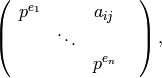
where
 and exactly of the
  are equal to
and
are equal to
and unless
  and
and  , in which case
 satisfies
  .
.
Remark A.19
The number of coset representatives for the operator is the
same as the number of points in the finite Grassmannian  . A similar phenomenon is true for the Hecke operators for
any group , although there are some subtleties [Gro98].
. A similar phenomenon is true for the Hecke operators for
any group , although there are some subtleties [Gro98].
A.4.3
Recall that in Section A.3.6 we constructed the Voronoi
decomposition and the well-rounded retract and that we can
use them to compute the cohomology  .
Unfortunately, we cannot directly use them to compute the action of the
Hecke operators on cohomology, since the Hecke operators do not act
cellularly on or . The problem is that the Hecke image of a
cell in (or ) is usually not a union of cells in (or
). This is already apparent for . The edges of are the
-translates of the ideal geodesic
.
Unfortunately, we cannot directly use them to compute the action of the
Hecke operators on cohomology, since the Hecke operators do not act
cellularly on or . The problem is that the Hecke image of a
cell in (or ) is usually not a union of cells in (or
). This is already apparent for . The edges of are the
-translates of the ideal geodesic  from to
(Example Example A.15). Applying a Hecke operator takes such an
edge to a union of ideal geodesics, each with vertices at a pair of
cusps. In general such geodesics are not an -translate
of .
from to
(Example Example A.15). Applying a Hecke operator takes such an
edge to a union of ideal geodesics, each with vertices at a pair of
cusps. In general such geodesics are not an -translate
of .
For , one solution is to work with all possible ideal geodesics
with vertices at the cusps, in other words the space of modular
symbols  from Section Modular Symbols. Manin’s trick (Proposition
Proposition 3.11) shows how to write any modular symbol as a
linear combination of unimodular symbols, by which we mean modular
symbols supported on the edges of . These are the ideas we now
generalize to all .
from Section Modular Symbols. Manin’s trick (Proposition
Proposition 3.11) shows how to write any modular symbol as a
linear combination of unimodular symbols, by which we mean modular
symbols supported on the edges of . These are the ideas we now
generalize to all .
Definition A.20
Let  be the -vector space
spanned by the symbols
be the -vector space
spanned by the symbols ![\vv = [v_{1},\dotsc ,v_{n}]](_images/math/2d669db6f59befd8c83d3368dde0631d5382de67.png) , where
, where  , modulo the following relations:
If
is a permutation on letters, then![[v_{1},\ldots,v_{n}] = \sign (\tau ) [\tau (v_{1}),\ldots,\tau
(v_{n})],](_images/math/465e23c383af4e5ed05e6e850850c627395914c3.png)
where
 is the sign of .
If
 , then
![[q v_{1},v_{2}\ldots,v_{n}] = [v_{1},\ldots,v_{n}].](_images/math/337b14dcdde2c2e5e068e21f44b05a155135e9e8.png)
If the points
 are linearly dependent, then
  .
.
Let  be the subspace generated by linear combinations
of the form
be the subspace generated by linear combinations
of the form
(14)![\sum _{i=0}^{n} (-1)^{i}
[v_{0},\ldots,\hat{v_{i}},\ldots,v_{n}],](_images/math/d44d238ba7dbebd5ada1114ed5b1b026ae64ebdf.png)
where  and where
  means to omit
  .
.
We call the space of modular symbols. We caution the
reader that there are some differences in what we call modular symbols
and those found in Section Modular Symbols and Definition
Definition 1.23; we compare them in
Section A.4.4. The group  acts on by
left multiplication:
acts on by
left multiplication: ![g\cdot \vv = [gv_{1},\dotsc ,gv_{n}]](_images/math/feff2df38b72216728e2096e8e09a0a200178b56.png) . This
action preserves the subspace and thus induces an action on the
quotient
. This
action preserves the subspace and thus induces an action on the
quotient  . For a finite
index subgroup, let
. For a finite
index subgroup, let  be the space of -coinvariants
in
be the space of -coinvariants
in  . In other words, is the quotient of by the
subspace generated by
. In other words, is the quotient of by the
subspace generated by  .
.
The relationship between modular symbols and the cohomology of
is given by the following theorem, first proved for
by Ash and Rudolph [AR79] and by Ash for general
[Ash86]:
Theorem A.21
Let be a
finite index subgroup. There is an isomorphism
(15)
where acts trivially on and where  .
.
We remark that Theorem A.21 remains true if is
replaced with nontrivial coefficients as in Section A.2.7.
Moreover, if is assumed to be torsion-free then we can
replace with  .
.
The great virtue of is that it admits an action of the
Hecke operators. Given a Hecke operator , write
the double coset  as a disjoint union of left cosets
(16)
as in Example A.18.
Any class in can be lifted to a representative  , where
  and almost all
  vanish.
Then we define
vanish.
Then we define
(17)
and extend to  by linearity. The right side of
(17) depends on the choices of and ,
but after taking quotients and coinvariants, we obtain a well-defined
action on cohomology via (15).
by linearity. The right side of
(17) depends on the choices of and ,
but after taking quotients and coinvariants, we obtain a well-defined
action on cohomology via (15).
A.4.4
The space is closely related to the space from
Section Modular Symbols and Section Modular Symbols. Indeed, was
defined to be the quotient  , where is
the free abelian group generated by ordered pairs
, where is
the free abelian group generated by ordered pairs
(18)
and is the subgroup generated by elements of the form
(19)
The only new feature in Definition Definition A.20 is item
(?). For this corresponds to the condition  , which follows from (19).
We have
, which follows from (19).
We have
Hence there are two differences between and : our
notion of modular symbols uses rational coefficients instead of
integral coefficients and is the space of symbols before
dividing out by the subspace of relations ; we further caution the
reader that this is somewhat at
odds with the literature.
We also remark that the general arbitrary weight definition of modular
symbols for a subgroup  given in
Section Modular Symbols also includes taking -coinvariants, as
well as extra data for a coefficient system. We have not included the
latter data since our emphasis is trivial coefficients, although it
would be easy to do so in the spirit of Section Modular Symbols.
given in
Section Modular Symbols also includes taking -coinvariants, as
well as extra data for a coefficient system. We have not included the
latter data since our emphasis is trivial coefficients, although it
would be easy to do so in the spirit of Section Modular Symbols.
Elements of also have a geometric interpretation: the symbol
 corresponds to the ideal geodesic in with
endpoints at the cusps
corresponds to the ideal geodesic in with
endpoints at the cusps  and
and  . We have a similar
picture for the symbols . We can assume
that each is primitive, which means that each
determines a vertex of the Voronoi polyhedron . The rational cone
generated by these vertices determines a subset
. We have a similar
picture for the symbols . We can assume
that each is primitive, which means that each
determines a vertex of the Voronoi polyhedron . The rational cone
generated by these vertices determines a subset  , where is the linear model of the symmetric space
  from Section A.3.2. This subset
  is
then an “ideal simplex” in . There is also a connection between
and torus orbits in ; we refer to [Ash86]
for a related discussion.
is
then an “ideal simplex” in . There is also a connection between
and torus orbits in ; we refer to [Ash86]
for a related discussion.
A.4.5
Now we need a generalization of the Manin trick (Section Computing with Modular Symbols). This is known in the literature as the modular symbols algorithm.
We can define a kind of norm function on as follows. Let ![\vv
=[v_{1},\dotsc ,v_{n}]](_images/math/5698feff07e246a98ca1f6c55d105ea50aeef1be.png) be a modular symbol. For each ,
choose
be a modular symbol. For each ,
choose  such that
  is
primitive. Then we define
is
primitive. Then we define

Note that  is well defined, since the
  are
unique up to sign, and permuting the only changes the
determinant by a sign. We extend
are
unique up to sign, and permuting the only changes the
determinant by a sign. We extend  to all of
by taking the maximum of over the support of any
to all of
by taking the maximum of over the support of any
 : if
: if  , where
and almost all vanish, then we put
, where
and almost all vanish, then we put
We say a modular symbol is unimodular if
 . It is clear that the images of the unimodular symbols generate
a finite-dimensional subspace of . The next theorem shows
that this subspace is actually all of
. It is clear that the images of the unimodular symbols generate
a finite-dimensional subspace of . The next theorem shows
that this subspace is actually all of  .
.
Theorem A.22
The space is spanned by
the images of the unimodular symbols. More precisely, given any symbol  with
with
 ,
,
in
 we may write
(20)
where if
 , then
  , and
, andthe number of terms on the right side of (20) is bounded by a polynomial in
 that depends only on the dimension .
Proof
(Sketch)
Given a modular symbol ![\vv =[v_{1},\dotsc ,v_{n}]](_images/math/3d36eb71c9757609c2902b1db7a2efd9759c6607.png) , we may assume
that the points are primitive. We will show that if
, we can find a point
, we may assume
that the points are primitive. We will show that if
, we can find a point  such that when we apply the
relation (14) using the points
such that when we apply the
relation (14) using the points  , all
terms other than
, all
terms other than  have norm less than . We call such
a point a reducing point for .
have norm less than . We call such
a point a reducing point for .
Let  be the open parallelotope
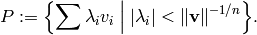
Then  is an -dimensional centrally symmetric convex body with
volume
is an -dimensional centrally symmetric convex body with
volume  . By Minkowski’s theorem from the geometry of numbers
(cf. [FT93, IV.2.6]),
. By Minkowski’s theorem from the geometry of numbers
(cf. [FT93, IV.2.6]),  contains a nonzero point
.
Using (14), we find
contains a nonzero point
.
Using (14), we find
(21)
where  is the symbol
![\vv_{i} (u) = [v_{1},\dotsc ,v_{i-1},u, v_{i+1},\dotsc ,v_{n}].](_images/math/312f2b8296a00ff67a7740932f06828906391c5a.png)
Moreover, it is easy to see that the new symbols satisfy
(22)
This completes the proof of the first statement.
To prove the second statement, we must estimate how many times
relations of the form (21) need to be applied to obtain
(20). A nonunimodular symbol produces at most new
modular symbols after (21) is performed; we potentially have
to apply (21) again to each of the symbols that result, which
in turn could produce as many as new symbols for each. Hence we
can visualize the process of constructing (20) as building
a rooted tree, where the root is , the leaves are the symbols
 , and where each node has at most children. It is not hard
to see that the bound (22) implies that the depth of this
tree (i.e., the longest length of a path from the root to a leaf) is
, and where each node has at most children. It is not hard
to see that the bound (22) implies that the depth of this
tree (i.e., the longest length of a path from the root to a leaf) is
 . From this the second statement follows
easily.
. From this the second statement follows
easily.
Statement (1) of Theorem A.22 is due to Ash and Rudolph
[AR79]. Instead of , they used the larger
parallelotope  defined by
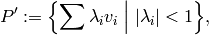
which has volume  . The observation that can be
replaced by and the proof of (2) are both due to Barvinok
[Bar94].
. The observation that can be
replaced by and the proof of (2) are both due to Barvinok
[Bar94].
A.4.6
The relationship between Theorem A.22 and Manin’s
trick should be clear. For , the Manin
symbols correspond exactly to the unimodular symbols mod . So
Theorem A.22 implies that every modular symbol (in the
language of Section Modular Symbols) is a linear combination of Manin
symbols. This is exactly the conclusion of Proposition
Proposition 1.24.
In higher rank the relationship between Manin symbols and unimodular
symbols is more subtle. In fact there are two possible notions of
“Manin symbol,” which agree for but not in general.
One possibility is the obvious one: a Manin symbol is a unimodular
symbol.
The other possibility is to define a Manin symbol to be a modular
symbol corresponding to a top-dimensional cell of the retract .
But for  , such modular symbols need not be unimodular. In
particular, for
, such modular symbols need not be unimodular. In
particular, for  there are two equivalence classes of
top-dimensional cells. One class corresponds to the unimodular
symbols, the other to a set of modular symbols of norm . However,
Theorems Theorem A.21 and Theorem A.22 show that
there are two equivalence classes of
top-dimensional cells. One class corresponds to the unimodular
symbols, the other to a set of modular symbols of norm . However,
Theorems Theorem A.21 and Theorem A.22 show that
 is spanned by unimodular symbols. Thus as far
as this cohomology group is concerned, the second class of symbols is
in some sense unnecessary.
is spanned by unimodular symbols. Thus as far
as this cohomology group is concerned, the second class of symbols is
in some sense unnecessary.
A.4.7
We return to the setting of Section A.3.8 and give
examples of Hecke eigenclasses in the cusp cohomology of  . We closely follow
[AGG84, vGvdKTV97].
Note that since the top of the cuspidal range for
. We closely follow
[AGG84, vGvdKTV97].
Note that since the top of the cuspidal range for
 is the same
as the virtual cohomological dimension , we can use modular
symbols to compute the Hecke action on cuspidal classes.
is the same
as the virtual cohomological dimension , we can use modular
symbols to compute the Hecke action on cuspidal classes.
Given a prime  coprime to , there are two Hecke operators of
interest
coprime to , there are two Hecke operators of
interest  and
and  . We can compute the action of these
operators on
. We can compute the action of these
operators on  as follows. Recall
that can be identified with a
certain space of functions
as follows. Recall
that can be identified with a
certain space of functions  (Theorem A.16). Given
  , let
, let  be a matrix such that
  under the
identification
under the
identification  . Then
  determines a unimodular symbol
 ![[Q_{x}]](_images/math/01cbc39edd8601d575c57918c0849de8f2b4c4f4.png) by taking the to be the columns of . Given any Hecke
operator , we can find coset representatives
by taking the to be the columns of . Given any Hecke
operator , we can find coset representatives  such that
 (explicit representatives
for
(explicit representatives
for  and
and  are given in
[AGG84, vGvdKTV97]). The modular symbols
are given in
[AGG84, vGvdKTV97]). The modular symbols ![[h_{i}Q_{x}]](_images/math/7a094aa34a3d984581a89dd48bbd544604cd663c.png) are no
longer unimodular in general, but we can apply Theorem
Theorem A.22 to write
are no
longer unimodular in general, but we can apply Theorem
Theorem A.22 to write
![[h_{i}Q_{x}] = \sum_{j} [R_{ij}], \quad R_{ij}\in \SL_{3} (\Z).](_images/math/fff064940ec6fa1e651d7ca34d36827a751df76e.png)
Then for  as in Theorem
Theorem A.16, we have
as in Theorem
Theorem A.16, we have
where  is the class of
  in
in  .
.
Now let  be a simultaneous
eigenclass for all the Hecke operators , , as
ranges over all primes coprime with . General considerations from
the theory of automorphic forms imply that the eigenvalues
be a simultaneous
eigenclass for all the Hecke operators , , as
ranges over all primes coprime with . General considerations from
the theory of automorphic forms imply that the eigenvalues  ,
,
 are complex conjugates of one other. Hence it suffices to
compute . We give two examples
of cuspidal eigenclasses for two different prime levels.
are complex conjugates of one other. Hence it suffices to
compute . We give two examples
of cuspidal eigenclasses for two different prime levels.
Example A.23
Let  . Then
  is
-dimensional. Let
is
-dimensional. Let  . One eigenclass is
given by the data
. One eigenclass is
given by the data
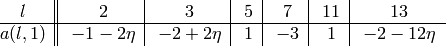
and the other is obtained by complex conjugation.
Example A.24
Let  . Then
  is
-dimensional. Let
is
-dimensional. Let  . One eigenclass is
given by the data
. One eigenclass is
given by the data

and the other is obtained by complex conjugation.
A.5 Other Cohomology Groups
A.5.1
In Section A.4 Hecke Operators and Modular Symbols we saw how to compute the Hecke action on
the top cohomology group  . Unfortunately for
 , this cohomology group does not contain any cuspidal
cohomology. The first case is
, this cohomology group does not contain any cuspidal
cohomology. The first case is  ; we have
 , and the cusp cohomology lives in degrees
  and
. One can show that the cusp cohomology in degree is dual to
that in degree , so for computational purposes it suffices to be
able to compute the Hecke action on
and
. One can show that the cusp cohomology in degree is dual to
that in degree , so for computational purposes it suffices to be
able to compute the Hecke action on  . But
modular symbols do not help us here.
. But
modular symbols do not help us here.
In this section we describe a technique to compute the Hecke action on
 , following [Gun00a]. The
technique is an extension of the modular symbol algorithm to these
cohomology groups. In principle the ideas in this section can be
modified to compute the Hecke action on other cohomology groups
, following [Gun00a]. The
technique is an extension of the modular symbol algorithm to these
cohomology groups. In principle the ideas in this section can be
modified to compute the Hecke action on other cohomology groups
 ,
,  , although this has not been
investigated [9]. For
, although this has not been
investigated [9]. For  , we have
applied the algorithm in joint work with Ash and McConnell to
investigate computationally the cohomology ,
where
, we have
applied the algorithm in joint work with Ash and McConnell to
investigate computationally the cohomology ,
where  [AGM02].
A.5.2
To begin, we need an analogue of Theorem A.21 for
lower degree cohomology groups. In other words, we need a
generalization of the modular symbols for other cohomology groups.
This is achieved by the sharbly complex  :
:
Definition A.25
Let
 be the chain complex given by the following data:
For
 ,
,  is the -vector space generated
by the symbols
is the -vector space generated
by the symbols ![\uu = [v_{1},\ldots,v_{n+k}]](_images/math/18e58873d1160ea0b22930f50642e0c347909b9d.png) , where , modulo the relations:
, where , modulo the relations:If
is a permutation on  letters, then
![[v_{1},\ldots,v_{n+k}] = \sign (\tau ) [\tau (v_{1}),\ldots,\tau
(v_{n+k})],](_images/math/f0655fe1967737abe65f76c7e62f9928438db779.png)
where
is the sign of .If
 , then
![[q v_{1},v_{2}\ldots,v_{n+k}] = [v_{1},\ldots,v_{n+k}].](_images/math/5d8f3d29b74eff993936dd69af8de82e68d3f0c2.png)
- If the rank of the matrix
 is less than , then
  .
.
For
 , the boundary map
  is
is![[v_{1},\ldots,v_{n+k}] \longmapsto \sum _{i=1}^{n+k} (-1)^{i}
[v_{1},\ldots,\hat{v_{i}},\ldots,v_{n+k}].](_images/math/8515d89fafa529f84a802658e6df6b8050705efe.png)
We define
 to be identically zero on .
The elements
![\uu = [v_{1},\dots ,v_{n+k}]](_images/math/ddb2f174b97e0b25fe8395920b469844c5e58231.png)
are called
-sharblies [10]. The -sharblies
are exactly the modular symbols from Definition
Definition A.20, and the subspace is the
image of the boundary map  .
.
There is an obvious left action of on  commuting
with . For any , let
commuting
with . For any , let  be the space
of -coinvariants. Since the boundary map commutes
with the -action, we obtain a complex
be the space
of -coinvariants. Since the boundary map commutes
with the -action, we obtain a complex  . The following theorem shows that this complex
computes the cohomology of :
. The following theorem shows that this complex
computes the cohomology of :
Theorem A.26
There is a natural isomorphism

We can extend our norm function  from modular
symbols to all of as follows. Let
from modular
symbols to all of as follows. Let ![\uu = [v_{1},\dots
,v_{n+k}]](_images/math/9e5a932ee20148a42a222d303799b1b739096e1f.png) be a -sharbly, and let
be a -sharbly, and let  be the set of all
submodular symbols determined by
be the set of all
submodular symbols determined by  . In other words,
  consists of the modular symbols of the form
 ![[v_{i_{1}},\dotsc
,v_{i_{n}}]](_images/math/3fec5d190180c694ed8b46f42097d243624869a9.png) , where
, where  ranges over all
-fold subsets of
ranges over all
-fold subsets of  . Define
  by
by
Note that  is well defined modulo the relations in
Definition Definition A.25. As for modular symbols, we extend
the norm to sharbly chains
is well defined modulo the relations in
Definition Definition A.25. As for modular symbols, we extend
the norm to sharbly chains  taking the maximum
norm over the support. Formally, we let
taking the maximum
norm over the support. Formally, we let  and
and  , and then we define
  by
by
We say that is reduced if  . Hence
is reduced if and only if all its submodular symbols are unimodular or
have determinant . Clearly there are only finitely many reduced
-sharblies modulo for any .
. Hence
is reduced if and only if all its submodular symbols are unimodular or
have determinant . Clearly there are only finitely many reduced
-sharblies modulo for any .
In general the cohomology groups are not
spanned by reduced sharblies. However, it is known (cf. [McC91])
that for  , the group
  is spanned by reduced -sharbly cycles. The best one can say
in general is that for each pair
is spanned by reduced -sharbly cycles. The best one can say
in general is that for each pair  , there is an integer
  such that for ,
  is spanned by -sharblies of norm
  . This set
of sharblies is also finite modulo , although it is not known
how large must be for any given pair .
. This set
of sharblies is also finite modulo , although it is not known
how large must be for any given pair .
A.5.4
Recall that the cells of the well-rounded retract are indexed by
sets of primitive vectors in . Since any primitive vector
determines a point in  and since sets of
such points index sharblies, it is clear that there is a close
relationship between and the chain complex associated to ,
although of course is much bigger. In any case, both
complexes compute .
and since sets of
such points index sharblies, it is clear that there is a close
relationship between and the chain complex associated to ,
although of course is much bigger. In any case, both
complexes compute .
The main benefit of using the sharbly complex to compute cohomology is
that it admits a Hecke action. Suppose  is a
sharbly cycle mod , and consider a Hecke operator .
Then we have
is a
sharbly cycle mod , and consider a Hecke operator .
Then we have
(23)
where is a set of coset representatives as in
(16).
Since  in general, the
Hecke image of a
reduced sharbly is not usually reduced.
in general, the
Hecke image of a
reduced sharbly is not usually reduced.
A.5.5
We are now ready to describe our algorithm for the computation of the
Hecke operators on  . It suffices to describe an
algorithm that takes as input a -sharbly cycle and produces
as output a cycle
. It suffices to describe an
algorithm that takes as input a -sharbly cycle and produces
as output a cycle  with
with
- the classes of and in
 the same, and
  if
if  .
.
Below, we will present an algorithm satisfying (a). In
[Gun00a], we conjectured (and presented evidence) that the
algorithm satisfies (b) for  . Further evidence is provided
by the computations in [AGM02], which relied on the
algorithm to compute the Hecke action on , where
. Further evidence is provided
by the computations in [AGM02], which relied on the
algorithm to compute the Hecke action on , where
 .
.
The idea behind the algorithm is simple: given a -sharbly cycle
that is not reduced, (i) simultaneously apply the modular symbol
algorithm (Theorem A.22) to each of its submodular
symbols, and then (ii) package the resulting data into a new -sharbly
cycle. Our experience in presenting this algorithm is that most
people find the geometry involved in (ii) daunting. Hence we will
give details only for and will provide a sketch for .
Full details are contained in [Gun00a]. Note that is
topologically and arithmetically uninteresting, since we are computing
the Hecke action on  ; nevertheless, the geometry
faithfully represents the situation for all .
; nevertheless, the geometry
faithfully represents the situation for all .
A.5.6
Fix , let  be a -sharbly cycle mod for
some
be a -sharbly cycle mod for
some  , and suppose is not
reduced. Assume is torsion-free to simplify the
presentation.
, and suppose is not
reduced. Assume is torsion-free to simplify the
presentation.
Suppose first that all submodular symbols  are
nonunimodular. Select reducing points for each
and make these choices -equivariantly. This means the
following. Suppose
are
nonunimodular. Select reducing points for each
and make these choices -equivariantly. This means the
following. Suppose  and
and
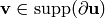 and
and  are modular
symbols such that
are modular
symbols such that  for some
  . Then we select reducing points for and
  for
for
 such that
  . (Note that since is
torsion-free, no modular symbol can be identified to itself by an
element of ; hence
. (Note that since is
torsion-free, no modular symbol can be identified to itself by an
element of ; hence  .) This is possible
since if is a modular symbol and is a reducing point for
, then
.) This is possible
since if is a modular symbol and is a reducing point for
, then  is a reducing point for
 for any . Because there are only finitely
many -orbits in
for any . Because there are only finitely
many -orbits in  , we can choose reducing points
-equivariantly by selecting them for some set of orbit
representatives.
, we can choose reducing points
-equivariantly by selecting them for some set of orbit
representatives.
It is important to note that -equivariance is the only
global criterion we use when selecting reducing. In
particular, there is a priori no relationship among the three reducing
points chosen for any  .
.
A.5.7
Now we want to use the reducing points and the -sharblies in to
build . Choose ![\uu = [v_{1},v_{2},v_{3}]\in
\support \xi](_images/math/101775efcba6c896a80918844ac2db1b1780f07a.png) , and denote the reducing point for
, and denote the reducing point for ![[v_{i},v_{j}]](_images/math/c7d988f853eaeb2ef594d9663b4e58f36bc55d76.png) by
by  ,
where
,
where  . We use the and the
 to build a -sharbly chain
  as follows.
Let be an octahedron in  . Label the vertices of with
the and such that the vertex labeled is
opposite the vertex labeled (Figure A.6).
Subdivide into four tetrahedra by connecting two opposite
vertices, say
. Label the vertices of with
the and such that the vertex labeled is
opposite the vertex labeled (Figure A.6).
Subdivide into four tetrahedra by connecting two opposite
vertices, say  and
and  , with an edge
(Figure A.7).
For each tetrahedron
, with an edge
(Figure A.7).
For each tetrahedron  , take the labels of four vertices and arrange
them into a quadruple. If we orient , then we can use the induced
orientation on to order the four primitive points. In this way,
each determines a -sharbly, and
, take the labels of four vertices and arrange
them into a quadruple. If we orient , then we can use the induced
orientation on to order the four primitive points. In this way,
each determines a -sharbly, and  is defined to be
the sum. For example, if we use the decomposition in
Figure A.7, we have
is defined to be
the sum. For example, if we use the decomposition in
Figure A.7, we have
(24)![\eta (\uu ) = [v_{1},v_{3},
v_{2},w_{1}]+[v_{1},w_{2},v_{3},w_{1}]+[v_{1},w_{3},w_{2},w_{1}]+[v_{1},v_{2},w_{3},w_{1}].](_images/math/b23d2582d27c5c4a28b6923e3e217b820ba6d28f.png)
Repeat this construction for all , and let
 . Finally, let
  .
.
Figure A.6
Figure A.7
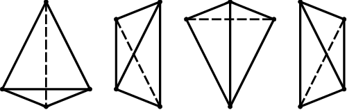
A.5.8
By construction,  is a cycle mod in the same
class as . We claim in addition that no submodular symbol from
appears in . To see this, consider
is a cycle mod in the same
class as . We claim in addition that no submodular symbol from
appears in . To see this, consider
 . From (24), we have
![\begin{multline}\label{bound}
\partial \eta (\uu ) = - [v_{1},v_{2},v_{3}] + [v_{1},v_{2},w_{3}] +
[v_{1},w_{2},v_{3}] + [w_{1},v_{2},v_{3}] \\
- [v_{1},w_{2},w_{3}] -
[w_{1},v_{2},w_{3}] - [w_{1},w_{2},v_{3}] + [w_{1},w_{2},w_{3}].
\end{multline}](_images/math/4868fd2348519e63f289465a2c181f0d1fa4c5bb.png)
Note that this is the boundary in , not in  .
Furthermore,
.
Furthermore,  is independent of which pair of
opposite vertices of we connected to build .
is independent of which pair of
opposite vertices of we connected to build .
From (?), we see that in  the
-sharbly
the
-sharbly ![-[v_{1},v_{2},v_{3}]](_images/math/969a6d318141fb73211b0b41f38fdf939e331991.png) is canceled by
. We also claim that
-sharblies in (?) of the form
is canceled by
. We also claim that
-sharblies in (?) of the form
![[v_{i},v_{j},w_{k}]](_images/math/07e00ef5b2456385302be0564faebf804c0f1ff2.png) vanish in
vanish in
 .
.
To see this, let  , and suppose
 ![\vv =
[v_{1},v_{2}]\in \support \partial \uu](_images/math/dfa6938d7683a6a1fbd9985982ca909dedf2a386.png) equals
equals  for some
 ![\vv ' = [v_{1}',v_{2}']\in \support \partial \uu'](_images/math/3a5244f3e49b772f59053d5b9e449c21b4b152ea.png) . Since
the reducing points were chosen -equivariantly, we have
. Since
the reducing points were chosen -equivariantly, we have
 . This means that the -sharbly
 ![[v_{1},v_{2},
w]\in \partial \eta (\uu )](_images/math/e0bb177cc2dbd1b4ebc6ee21a966f2aa53033575.png) will be canceled mod by
will be canceled mod by
![[v_{1}',v_{2}', w']\in \partial \eta (\uu' )](_images/math/17feb974f78197cc400249844cb7ad6f7cf8e282.png) . Hence, in passing
from to , the effect in
. Hence, in passing
from to , the effect in  is to replace
with four -sharblies in
is to replace
with four -sharblies in  :
:
(25)![[v_{1},v_{2},v_{3}]\longmapsto - [v_{1},w_{2},w_{3}] -
[w_{1},v_{2},w_{3}] - [w_{1},w_{2},v_{3}] + [w_{1},w_{2},w_{3}].](_images/math/4613808aff707bd09d6ebec5bead65a0a59abd71.png)
Note that in (25), there are no -sharblies of the form
.
Remark A.27
For implementation purposes, it is not necessary to explicitly
construct . Rather, one may work directly with (25).
A.5.9
Why do we expect to satisfy  ? First of
all, in the right hand side of (25) there are no submodular
symbols of the form . In fact, any submodular symbol
involving a point also includes a reducing point for
.
? First of
all, in the right hand side of (25) there are no submodular
symbols of the form . In fact, any submodular symbol
involving a point also includes a reducing point for
.
On the other hand, consider the submodular symbols in (25) of
the form ![[w_{i},w_{j}]](_images/math/d841a06859d132bebff94f85e54ca6ad7a6bc9ca.png) . Since there is no relationship among the
, one has no reason to believe that these modular symbols are
closer to unimodularity than those in . Indeed, for certain
choices of reducing points it can happen that
. Since there is no relationship among the
, one has no reason to believe that these modular symbols are
closer to unimodularity than those in . Indeed, for certain
choices of reducing points it can happen that ![\|[w_{i},w_{j}]\|\geq
\|\uu \|](_images/math/efb72005863e3ad454b2452e1f65294e1907648e.png) .
.
The upshot is that some care must be taken in choosing reducing
points. In [Gun00a, Conjectures 3.5 and 3.6] we describe
two methods for finding reducing points for modular symbols, one using
Voronoi reduction and one using LLL-reduction. Our experience is that
if one selects reducing points using either of these conjectures,
then ![\|[w_{i},w_{j}]\|< \|\uu \|](_images/math/c03c2fd4d1b66f58945ab8e2f5ff87b9abb85f20.png) for each of the new modular symbols
. In fact, in practice these symbols are trivial or
satisfy
for each of the new modular symbols
. In fact, in practice these symbols are trivial or
satisfy ![\|[w_{i},w_{j}]\|=1](_images/math/9e40224cdb9d1bbed7e01fa03b8be5c8f4ca2fd8.png) .
.
A.5.10
In the previous discussion we assumed that no submodular symbols of
any were unimodular. Now we say what to
do if some are. There are three cases to consider.
First, all submodular symbols of may be unimodular. In this
case there are no reducing points, and (25) becomes
(26)![[v_{1},v_{2},v_{3}]\longmapsto [v_{1},v_{2},v_{3}].](_images/math/044a5b2eab7a2ebf7bd5606cc0ccf07847e3b50d.png)
Second, one submodular symbol of may be nonunimodular, say the
symbol ![[v_{1},v_{2}]](_images/math/b9809b93d13bfe32cb03bd0ac2504c17dcf1e243.png) . In this case, to build , we use a
tetrahedron
and put
. In this case, to build , we use a
tetrahedron
and put ![\eta (\uu ) = [v_{1},v_{2},v_{3},w_{3}]](_images/math/18e6a5a670c61b098810adef88e1ee576ec90523.png) (Figure A.8). Since
(Figure A.8). Since ![[v_{1}, v_{2}, w_{3}]](_images/math/4b65be36d11b2f54aeae2afe9d1bae02159345ba.png) vanishes
in the boundary of mod , (25) becomes
vanishes
in the boundary of mod , (25) becomes
(27)![[v_{1},v_{2},v_{3}]\mapsto -[v_{1},v_{3},w_{3}] + [v_{2}, v_{3},
w_{3}].](_images/math/3adc0761f8d693d145d79d19722d4f136139cadd.png)
Figure A.8
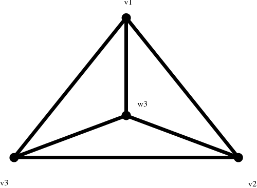
Finally, two submodular symbols of may be nonunimodular, say
and ![[v_{1},v_{3}]](_images/math/4e258e4bc34edf9b2d1255f9037726a4f1efad56.png) . In this case we use the cone on
a square
. In this case we use the cone on
a square  (Figure A.9). To construct
  , we must choose a decomposition of into tetrahedra.
Since has a nonsimplicial face, this choice affects (in
contrast to the previous cases). If we subdivide by connecting
the vertex labelled
, we must choose a decomposition of into tetrahedra.
Since has a nonsimplicial face, this choice affects (in
contrast to the previous cases). If we subdivide by connecting
the vertex labelled  with the vertex labelled
  , we
obtain
, we
obtain
(28)![[v_{1},v_{2},v_{3}]\longmapsto[v_{2},w_{2},w_{3}]+[v_{2},v_{3},w_{2}]+
[v_{1},v_{3},w_{2}].](_images/math/08e7eab9fdcdffbafabe798fcafd49d7b53715e7.png)
Figure A.9
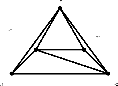
A.5.11
Now consider general . The basic technique is the same, but the
combinatorics become more complicated. Suppose ![\uu = [v_{1},\dots ,v_{n+1}]](_images/math/9edd320983d727e5d8a4ad05d6aab029abce9027.png) satisfies
satisfies  in a -sharbly cycle , and for
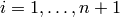 let
let  be the submodular symbol
![[v_{1},\dots,\widehat{v_{i}},\dots ,v_{n+1}]](_images/math/65054f8833f42eb8b67250f8b3d68081b8bdde9f.png) . Assume that all are
nonunimodular, and for each let be a reducing point for
.
. Assume that all are
nonunimodular, and for each let be a reducing point for
.
For any subset  , let
, let  be the
-sharbly
be the
-sharbly ![[u_{1},\dots ,u_{n+1}]](_images/math/99962bee7612b36edbeee348475be3a5400c7621.png) , where
, where  if
if  ,
and
,
and  otherwise. The polytope used to build
  is the cross polytope, which is the higher-dimensional
analogue of the octahedron [Gun00a, Section 4.4]. We suppress the
details and give the final answer:
(25) becomes
is the cross polytope, which is the higher-dimensional
analogue of the octahedron [Gun00a, Section 4.4]. We suppress the
details and give the final answer:
(25) becomes
(29)
where the sum is taken over all subsets  of cardinality at least `2`.
More generally, if some happen to be unimodular, then the
polytope used to build is an iterated cone on a
lower-dimensional cross polytope. This is already visible for :
- The 2-dimensional cross polytope is a
square, and the polytope is
a cone on a square.
- The 1-dimensional cross polytope is an interval, and the
polytope is a double cone on an interval.
 relations generalizing
A.5.12
Now we describe how these computations are carried out in practice,
focusing on and  . Besides discussing technical details,
we also have to slightly modify some aspects of the construction in
Section A.5.6, since is not torsion-free.
. Besides discussing technical details,
we also have to slightly modify some aspects of the construction in
Section A.5.6, since is not torsion-free.
Let be the well-rounded retract. We can represent
a cohomology class
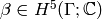 as
as
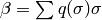 , where denotes a codimension
cell in . In this case there are three types of codimension
cells in . Under the bijection
, where denotes a codimension
cell in . In this case there are three types of codimension
cells in . Under the bijection  , these cells
correspond to the Voronoi cells indexed by the columns of the matrices
, these cells
correspond to the Voronoi cells indexed by the columns of the matrices
(30)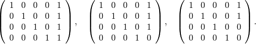
Thus each in modulo corresponds to an  -translate of one of the matrices in (30).
These translates
determine basis -sharblies (by taking the points
-translate of one of the matrices in (30).
These translates
determine basis -sharblies (by taking the points  to
be the columns), and hence we can represent by a 1-sharbly
chain
to
be the columns), and hence we can represent by a 1-sharbly
chain 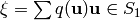 that is a cycle in the complex of coinvariants
 .
.
To make later computations more efficient, we precompute more data
attached to . Given a -sharbly ![\uu = [u_{1},\dotsc
,u_{n+1}]](_images/math/eaf2c81ad0e976db9067da2e8b3a4e04dafd462a.png) , a lift
, a lift  of is defined to be an
integral matrix with primitive columns
of is defined to be an
integral matrix with primitive columns  such that
 ![\uu =
[M_{1},\dotsc ,M_{n+1}]](_images/math/0b8611718c9583afef8bcd6a62a5474592ac20c9.png) . Then we encode , once and for all, by
a finite collection
. Then we encode , once and for all, by
a finite collection  of -tuples
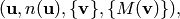
where
- ranges over the support of ,
 is the coefficient of in ,
 is the set of submodular symbols appearing in the
boundary of , and
is the set of submodular symbols appearing in the
boundary of , and is a set of lifts for .
Moreover, the lifts in (4) are chosen to satisfy the
following -equivariance condition. Suppose that for
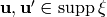 we have
and
we have
and  satisfying
 for some . Then we require
  . This is possible since is a cycle modulo
, although there is one complication since has torsion:
it can happen that some submodular symbol
of a -sharbly is identified to itself by an
element of .
This means that in constructing
. This is possible since is a cycle modulo
, although there is one complication since has torsion:
it can happen that some submodular symbol
of a -sharbly is identified to itself by an
element of .
This means that in constructing  for , we must somehow choose more than one lift for .
To deal with this, let
for , we must somehow choose more than one lift for .
To deal with this, let  be any lift of , and let
  be
the stabilizer of . Then in , we replace
be
the stabilizer of . Then in , we replace  by
by
where  has the same data as ,
except [11]
that we give
the lift
has the same data as ,
except [11]
that we give
the lift  .
.
Next we compute and store the 1-sharbly transformation laws generalizing (26)–(28). As a part of this we fix triangulations of certain cross polytopes as in (28).
We are now ready to begin the actual reduction algorithm. We take a
Hecke operator  and build the coset representatives
as in (23). For each
and build the coset representatives
as in (23). For each  and each
-sharbly in the support of , we obtain a non-reduced
-sharbly
and each
-sharbly in the support of , we obtain a non-reduced
-sharbly  . Here
  acts on all the data
attached to in the list . In particular, we replace each
lift
acts on all the data
attached to in the list . In particular, we replace each
lift  with
with  , where the dot means matrix
multiplication.
, where the dot means matrix
multiplication.
Now we check the submodular symbols of  and choose reducing
points for the nonunimodular symbols. This is where the lifts come in
handy. Recall that reduction points must be chosen
-equivariantly over the entire cycle. Instead of explicitly
keeping track of the identifications between modular symbols, we do
the following trick:
and choose reducing
points for the nonunimodular symbols. This is where the lifts come in
handy. Recall that reduction points must be chosen
-equivariantly over the entire cycle. Instead of explicitly
keeping track of the identifications between modular symbols, we do
the following trick:
- Construct the Hermite normal form
 of the lift (see [Coh93, Section 2.4] and Exercise 7.5). Record the transformation matrix
  such
that
such
that  .
. - Choose a reducing point for
 .
.
3. Then the reducing point for is  .
This guarantees -equivariance: if ,
.
This guarantees -equivariance: if ,  are submodular
symbols of with
are submodular
symbols of with  and with reducing
points
and with reducing
points  , we have
  . The reason is that the
Hermite normal form is a uniquely determined
representative of the
. The reason is that the
Hermite normal form is a uniquely determined
representative of the  -orbit of
[Coh93]. Hence if
-orbit of
[Coh93]. Hence if  , then
  .
.
After computing all reducing points, we apply the appropriate
transformation law. The result will be a chain of -sharblies, each
of which has (conjecturally) smaller norm than the original
-sharbly . We output these -sharblies if they are reduced;
otherwise they are fed into the reduction algorithm again. Eventually
we obtain a reduced -sharbly cycle homologous to the
original cycle .
The final step of the algorithm is to rewrite as a cocycle on
. This is easy to do since the relevant cells of are in
bijection with the reduced -sharblies. There are some nuisances in
keeping orientations straight, but the computation is not difficult.
We refer to [AGM02] for details.
A.5.13
We now give some examples, taken from [AGM02], of Hecke
eigenclasses in  for various levels
.
Instead of giving a table of eigenvalues, we give the Hecke polynomials.
If is an eigenclass with
for various levels
.
Instead of giving a table of eigenvalues, we give the Hecke polynomials.
If is an eigenclass with
 , then we define
![H (\beta , l) = \sum_k (-1)^k l^{k(k-1)/2} a(l, k) X^k \in \C [X].](_images/math/46e48f119ab889f84fdd7ac5c81cb606011637d7.png)
For almost all , after putting  where is a complex
variable, the function
where is a complex
variable, the function  is the inverse of the local factor at of the
automorphic representation attached to .
is the inverse of the local factor at of the
automorphic representation attached to .
Example A.28
Suppose  . Then the cohomology
 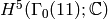 is
2-dimensional. There are two Hecke eigenclasses
is
2-dimensional. There are two Hecke eigenclasses  , each
with rational Hecke eigenvalues.
, each
with rational Hecke eigenvalues.
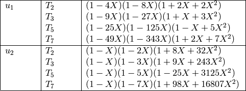
Example A.29
Suppose  . Then the cohomology
 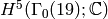 is 3-dimensional. There are three Hecke
eigenclasses
is 3-dimensional. There are three Hecke
eigenclasses  , each with rational Hecke
eigenvalues.
, each with rational Hecke
eigenvalues.
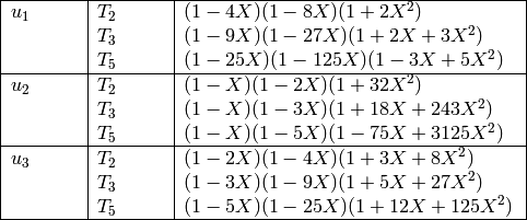
In these examples, the cohomology is completely accounted for by the
Eisenstein summand of (8). In fact, let
 be the usual Hecke congruence
subgroup of matrices upper-triangular modulo . Then the cohomology
classes above actually come from classes in
be the usual Hecke congruence
subgroup of matrices upper-triangular modulo . Then the cohomology
classes above actually come from classes in  ,
that is from holomorphic modular forms of level .
,
that is from holomorphic modular forms of level .
For , the space of weight two cusp forms  is
1-dimensional. This cusp form lifts in two different ways to
, which can be seen from the quadratic
part of the Hecke polynomials for the
is
1-dimensional. This cusp form lifts in two different ways to
, which can be seen from the quadratic
part of the Hecke polynomials for the  . Indeed, for the
quadratic part is exactly the inverse of the local factor for the
. Indeed, for the
quadratic part is exactly the inverse of the local factor for the
 -function attached to , after the substitution .
For
-function attached to , after the substitution .
For  , we see that the lift is also twisted by the square of the
cyclotomic character. (In fact the linear terms of the Hecke
polynomials come from powers of the cyclotomic character.)
, we see that the lift is also twisted by the square of the
cyclotomic character. (In fact the linear terms of the Hecke
polynomials come from powers of the cyclotomic character.)
For , the space of weight two cusp forms  is again
1-dimensional. The classes
is again
1-dimensional. The classes  and are lifts of this
form, exactly as for . The class
and are lifts of this
form, exactly as for . The class  , on the other hand,
comes from
, on the other hand,
comes from  , the space of weight cusp forms on
 . In fact,
  , with one Hecke
eigenform defined over and another defined over a totally real
cubic extension of . Only the rational weight four eigenform
contributes to
, with one Hecke
eigenform defined over and another defined over a totally real
cubic extension of . Only the rational weight four eigenform
contributes to  . One can show that
whether or not a weight four cuspidal eigenform contributes to the
cohomology of depends only on the sign of the
functional equation of
. One can show that
whether or not a weight four cuspidal eigenform contributes to the
cohomology of depends only on the sign of the
functional equation of  [Wes]. This phenomenon
is typical of what one encounters when studying Eisenstein cohomology.
[Wes]. This phenomenon
is typical of what one encounters when studying Eisenstein cohomology.
In addition to the lifts of weight 2 and weight 4 cusp forms, for
other levels one finds lifts of Eisenstein series of weights 2 and 4
and lifts of cuspidal cohomology classes from subgroups of  . For some levels one finds cuspidal classes that appear to be
lifts from the group of symplectic similitudes
. For some levels one finds cuspidal classes that appear to be
lifts from the group of symplectic similitudes  . More
details can be found in [AGM02, AGM].
. More
details can be found in [AGM02, AGM].
A.5.14
Here are some notes on the reduction algorithm and its implementation:
Some additional care must be taken when selecting reducing points for the submodular symbols of
. In particular, in
practice one should choose for such that  is minimized. Similar remarks apply when choosing a
subdivision of the crosspolytopes in Section A.5.10.
is minimized. Similar remarks apply when choosing a
subdivision of the crosspolytopes in Section A.5.10.In practice, the reduction algorithm has always terminated with a reduced
-sharbly cycle homologous to . However, at
the moment we cannot prove that this will always happen.Experimentally, the efficiency of the reduction step appears to be comparable to that of Theorem A.22. In other words the depth of the “reduction tree” associated to a given
-sharbly
seems to be bounded by a polynomial in  . Hence
computing the Hecke action using this algorithm is extremely
efficient.
. Hence
computing the Hecke action using this algorithm is extremely
efficient.On the other hand, computing Hecke operators on
 is still a
much bigger computation—relative to the level—than on
is still a
much bigger computation—relative to the level—than on  and . For example, the size of the full retract modulo
 is roughly
  , which grows rapidly with .
The portion of the retract corresponding to
, which grows rapidly with .
The portion of the retract corresponding to  is much smaller,
around
is much smaller,
around  , but this still grows quite quickly. This makes
computing with
, but this still grows quite quickly. This makes
computing with  out of reach at the moment.
The number of Hecke cosets grows rapidly as well, e.g., the number of coset representatives of
is  . Hence
it is only feasible to compute Hecke operators for small ; for
large levels only
. Hence
it is only feasible to compute Hecke operators for small ; for
large levels only  is possible.
Here are some numbers to give an idea of the size of these computations. For level
 , the rank of is 20. There are
39504 cells of codimension and 4128 top-dimensional cells in
modulo
, the rank of is 20. There are
39504 cells of codimension and 4128 top-dimensional cells in
modulo  . The computational techniques in
[AGM02] used at this level (a Lanczos scheme over a large
finite field) tend to produce sharbly cycles supported on almost all
the cells. Computing
. The computational techniques in
[AGM02] used at this level (a Lanczos scheme over a large
finite field) tend to produce sharbly cycles supported on almost all
the cells. Computing  requires a reduction tree of
depth
and produces as many as 26 reduced -sharblies for each of the 15
nonreduced Hecke images. Thus one cycle produces a cycle supported on
as many as 15406560 -sharblies, all of which must be converted to
an appropriate cell of modulo . Also this is just what
needs to be done for one cycle; do not forget that the rank of
is 20.
requires a reduction tree of
depth
and produces as many as 26 reduced -sharblies for each of the 15
nonreduced Hecke images. Thus one cycle produces a cycle supported on
as many as 15406560 -sharblies, all of which must be converted to
an appropriate cell of modulo . Also this is just what
needs to be done for one cycle; do not forget that the rank of
is 20.In practice the numbers are slightly better, since the reduction step produces fewer
-sharblies on average and since the support of the
initial cycle has size less than  . Nevertheless the orders of
magnitude are correct.
. Nevertheless the orders of
magnitude are correct.Using lifts is a convenient way to encode the global
-identifications in the cycle , since it means we do not
have to maintain a big data structure keeping track of the identifications on
 . However, there is a certain expense in computing the
Hermite normal form. This is balanced by the benefit that working
with the data associated to allows us to reduce the
supporting -sharblies independently. This means we
can cheaply parallelize our computation: each -sharbly, encoded as
a -tuple
. However, there is a certain expense in computing the
Hermite normal form. This is balanced by the benefit that working
with the data associated to allows us to reduce the
supporting -sharblies independently. This means we
can cheaply parallelize our computation: each -sharbly, encoded as
a -tuple 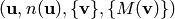 , can be
handled by a separate computer. The results of all these individual
computations can then be collated at the end, when producing a
-cocycle.
, can be
handled by a separate computer. The results of all these individual
computations can then be collated at the end, when producing a
-cocycle.
A.6 Complements and Open Problems
A.6.1
We conclude this appendix by giving some complements and describing some possible directions for future work, both theoretical and computational. Since a full explanation of the material in this section would involve many more pages, we will be brief and will provide many references.
A.6.2 Perfect Quadratic Forms over Number Fields and Retracts
Since Voronoi’s pioneering work [Vor08], it has been the goal of
many to extend his results from to a general algebraic number
field . Recently Coulangeon [Cou01], building on work of Icaza
and Baeza [Ica97, BI97], has found a good notion of
perfection for quadratic forms over number
fields [12]. One of the key ideas in [Cou01] is that the correct
notion of equivalence between Humbert forms involves not only the
action of  , where
  is the ring of integers
of , but also the action of a certain continuous group
is the ring of integers
of , but also the action of a certain continuous group  related
to the units
related
to the units  . One of Coulangeon’s basic results
is that there are finitely many equivalence classes of perfect Humbert
forms modulo these actions.
. One of Coulangeon’s basic results
is that there are finitely many equivalence classes of perfect Humbert
forms modulo these actions.
On the other hand, Ash’s original construction of retracts
[Ash77] introduces a geometric notion of perfection. Namely he
generalizes the Voronoi polyhedron and defines a quadratic form to
be perfect if it naturally indexes a facet of . What is the
connection between these two notions? Can one use Coulangeon’s
results to construct cell complexes to be used in cohomology
computations? One tempting possibility is to try to use the group
to collapse the Voronoi cells of [Ash77] into a
cell decomposition of the symmetric space associated to  .
.
A.6.3 The Modular Complex
In his study of multiple  -values, Goncharov has recently defined
the modular complex
-values, Goncharov has recently defined
the modular complex  [Gon97, Gon98]. This is an
-step complex of
[Gon97, Gon98]. This is an
-step complex of  -modules closely related both to the
properties of multiple polylogarithms evaluated at
-modules closely related both to the
properties of multiple polylogarithms evaluated at  , the
, the
 roots of unity, and to the action of
  on
on  , the
pro- completion of the algebraic fundamental group of
, the
pro- completion of the algebraic fundamental group of
 .
.
Remarkably, the modular complex is very closely related to the Voronoi
decomposition  . In fact, one can succinctly describe the modular
complex by saying that it is the chain complex of the cells coming
from the top-dimensional Voronoi cone of type . This is all of
the Voronoi decomposition for
. In fact, one can succinctly describe the modular
complex by saying that it is the chain complex of the cells coming
from the top-dimensional Voronoi cone of type . This is all of
the Voronoi decomposition for  , and Goncharov showed that the
modular complex is quasi-isomorphic to the full Voronoi complex for
. Hence there is a precise relationship among multiple
polylogarithms, the Galois action on
, and Goncharov showed that the
modular complex is quasi-isomorphic to the full Voronoi complex for
. Hence there is a precise relationship among multiple
polylogarithms, the Galois action on  , and the cohomology
of level congruence subgroups of .
, and the cohomology
of level congruence subgroups of .
The question then arises, how much of the cohomology of congruence
subgroups is captured by the modular complex for all ?
Table A.2 indicates that asymptotically very little of the Voronoi
decomposition comes from the  cone, but this says nothing about
the cohomology. The first interesting case to consider is .
cone, but this says nothing about
the cohomology. The first interesting case to consider is .
A.6.4 Retracts for Other Groups
The most general construction of retracts known [Ash84]
applies only to linear symmetric spaces.index{linear symmetric spaces}
The most familiar
example of such a space is  ; other examples are
the symmetric spaces associated to over number fields and
division algebras.
; other examples are
the symmetric spaces associated to over number fields and
division algebras.
Now let  be an arithmetic group, and let
  be the associated symmetric space. What can one say about cell
complexes that can be used to compute
be the associated symmetric space. What can one say about cell
complexes that can be used to compute  ? The
theorem of Borel–Serre mentioned in Section A.3.3 implies the
vanishing of
? The
theorem of Borel–Serre mentioned in Section A.3.3 implies the
vanishing of  for
for  , where
 is the -rank of . For example, for the split
form of , the -rank is . For the split symplectic
group , the -rank is . Moreover, this bound is
sharp: there will be coefficient modules for which
is the -rank of . For example, for the split
form of , the -rank is . For the split symplectic
group , the -rank is . Moreover, this bound is
sharp: there will be coefficient modules for which  . Hence any minimal cell complex used to compute the
cohomology of should have dimension .
. Hence any minimal cell complex used to compute the
cohomology of should have dimension .
Ideally one would like to see such a complex realized as a subspace of
and would like to be able to treat all finite index subgroups of
simultaneously. This leads to the following question: is
there a -equivariant deformation retraction of onto a
regular cell complex of dimension ?
For  , McConnell and MacPherson showed that the answer is
yes. Their construction begins by realizing the symplectic symmetric
space
, McConnell and MacPherson showed that the answer is
yes. Their construction begins by realizing the symplectic symmetric
space  as a subspace of the special linear symmetric space
 . They then construct subsets of by intersecting
the Voronoi cells in with . Through explicit
computations in coordinates they prove that these intersections are
cells and give a cell decomposition of . By taking an
appropriate dual complex (as suggested by Figure A.2 and
Figure A.3 and as done in [Ash77]), they construct the
desired cell complex .
. They then construct subsets of by intersecting
the Voronoi cells in with . Through explicit
computations in coordinates they prove that these intersections are
cells and give a cell decomposition of . By taking an
appropriate dual complex (as suggested by Figure A.2 and
Figure A.3 and as done in [Ash77]), they construct the
desired cell complex .
Other progress has been recently made by Bullock [Bul00],
Bullock and Connell [BC06], and Yasaki
[Yas05b, Yas05a] in the case of groups of -rank 1. In particular, Yasaki
uses the tilings of Saper [Sap97] to construct an explicit
retract for the unitary group  over the Gaussian integers.
His method also works for Hilbert modular groups, although further
refinement may be needed to produce a regular cell complex. Can one
generalize these techniques to construct retracts for groups of
arbitrary -rank? Is there an analogue of the Voronoi decomposition
for these retracts (i.e., a dual cell decomposition of the symmetric
space)? If so, can one generalize ideas in
Sections A.4 Hecke Operators and Modular Symbols – A.5 Other Cohomology Groups and use
that generalization to compute the
action of the Hecke operators on the cohomology?
over the Gaussian integers.
His method also works for Hilbert modular groups, although further
refinement may be needed to produce a regular cell complex. Can one
generalize these techniques to construct retracts for groups of
arbitrary -rank? Is there an analogue of the Voronoi decomposition
for these retracts (i.e., a dual cell decomposition of the symmetric
space)? If so, can one generalize ideas in
Sections A.4 Hecke Operators and Modular Symbols – A.5 Other Cohomology Groups and use
that generalization to compute the
action of the Hecke operators on the cohomology?
A.6.5 Deeper Cohomology Groups
The algorithm in Section A.5 Other Cohomology Groups can be used
to compute the Hecke action on
 . For
. For  , this group no longer contains
cuspidal cohomology classes. Can one generalize this algorithm to
compute the Hecke action on deeper cohomology groups? The first
practical case is . Here
, this group no longer contains
cuspidal cohomology classes. Can one generalize this algorithm to
compute the Hecke action on deeper cohomology groups? The first
practical case is . Here  , and the highest degree in
which cuspidal cohomology can live is
, and the highest degree in
which cuspidal cohomology can live is  . This case is also
interesting since the cohomology of full level has been studied
[EVGS02].
. This case is also
interesting since the cohomology of full level has been studied
[EVGS02].
Here are some indications of what one can expect. The general
strategy is the same: for a -sharbly representing a
class in  , begin by -equivariantly
choosing reducing points for the nonunimodular submodular symbols of
. This data can be packaged into a new -sharbly cycle as in
Section A.5.7, but the crosspolytopes must be replaced
with hypersimplices. By definition, the hypersimplex
, begin by -equivariantly
choosing reducing points for the nonunimodular submodular symbols of
. This data can be packaged into a new -sharbly cycle as in
Section A.5.7, but the crosspolytopes must be replaced
with hypersimplices. By definition, the hypersimplex  is the convex hull in of the points
  , where ranges over all order subsets of
  and
and  denotes the standard
basis of
denotes the standard
basis of  .
.
The simplest example is , . From the point of view of
cohomology, this is even less interesting than ,  , since now
we are computing the Hecke action on
, since now
we are computing the Hecke action on  ! Nevertheless,
the geometry here illustrates what one can expect in general.
! Nevertheless,
the geometry here illustrates what one can expect in general.
Each -sharbly in the support of can be written as
![[v_{1},v_{2},v_{3},v_{4}]](_images/math/febffaf8ddb51351f7149261590c18b61d7da009.png) and determines six submodular symbols, of
the form
and determines six submodular symbols, of
the form ![[v_{i}, v_{j}]](_images/math/fdb1a86e0ebf0c9afac27517f845b8fd3bad8ec8.png) ,
,  . Assume for simplicity that all these
submodular symbols are nonunimodular. Let
. Assume for simplicity that all these
submodular symbols are nonunimodular. Let  be the reducing
point for . Then use the ten points
be the reducing
point for . Then use the ten points  to
label the vertices of the hypersimplex
to
label the vertices of the hypersimplex  as in
Figure A.10 (note that is -dimensional).
as in
Figure A.10 (note that is -dimensional).
Figure A.10
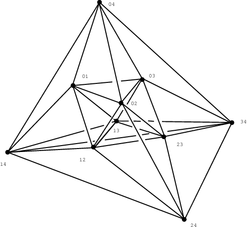
The boundary of this hypersimplex gives the analogue of
(25). Which -sharblies will appear in ? The boundary
 is a union of five tetrahedra and five octahedra.
The outer tetrahedron will not appear in , since that is the
analogue of the left side of (25). The four octahedra sharing a
triangular face with the outer tetrahedron also will not appear, since
they disappear when considering modulo . The
remaining four tetrahedra and the central octahedron survive to
and constitute the right side of the analogue of (25). Note that we
must choose a simplicial subdivision of the central octahedron to write
the result as a -sharbly cycle and that this must be done with
care since it introduces a new submodular symbol.
is a union of five tetrahedra and five octahedra.
The outer tetrahedron will not appear in , since that is the
analogue of the left side of (25). The four octahedra sharing a
triangular face with the outer tetrahedron also will not appear, since
they disappear when considering modulo . The
remaining four tetrahedra and the central octahedron survive to
and constitute the right side of the analogue of (25). Note that we
must choose a simplicial subdivision of the central octahedron to write
the result as a -sharbly cycle and that this must be done with
care since it introduces a new submodular symbol.
If some submodular symbols are unimodular, then again one must
consider iterated cones on hypersimplices, just as in
Section A.5.10. The analogues of these steps become more
complicated, since there are now many simplicial subdivisions of a
hypersimplex [13]. There is
one final complication: in general we cannot use reduced -sharblies
alone to represent cohomology classes. Thus one must terminate the
algorithm when is less than some predetermined bound.
A.6.6 Other Linear Groups
Let be a number field, and let  (Example A.2). Let
  be an
arithmetic subgroup. Can one compute the action of the
Hecke operators on
be an
arithmetic subgroup. Can one compute the action of the
Hecke operators on  ?
?
There are two completely different approaches to this problem. The first involves the generalization of the modular symbols method. One can define the analogue of the sharbly complex, and can try to extend the techniques of Sections A.4 Hecke Operators and Modular Symbols–A.5 Other Cohomology Groups.
This technique has been extensively used when
is imaginary quadratic and . We have  , which is isomorphic to -dimensional hyperbolic
space
, which is isomorphic to -dimensional hyperbolic
space  . The arithmetic groups
  are known as Bianchi groups. The retracts and
cohomology of these groups have been well studied; as a representative
sample of works we mention
[Men79, EGM98, Vog85, GS81].
are known as Bianchi groups. The retracts and
cohomology of these groups have been well studied; as a representative
sample of works we mention
[Men79, EGM98, Vog85, GS81].
Such groups have -rank 1 and thus have cohomological dimension
. One can show that the cuspidal classes live in degrees and
. This means that we can use modular symbols to investigate the
Hecke action on cuspidal cohomology. This was done by Cremona
[Cre84] for euclidean fields . In that case Theorem
Theorem A.22 works with no trouble (the euclidean algorithm is
needed to construct reducing points). For noneuclidean fields
further work has been done by Whitley [Whi90], Cremona and Whitely
[Cre97c] (both for principal ideal domains), Bygott
[Byg99] (for  and any field with class group
an elementary abelian -group), and Lingham [Lin05] (any
field with odd class number). Putting all these ideas together allows
one to generalize the modular symbols method to any imaginary
quadratic field [Cre].
and any field with class group
an elementary abelian -group), and Lingham [Lin05] (any
field with odd class number). Putting all these ideas together allows
one to generalize the modular symbols method to any imaginary
quadratic field [Cre].
For imaginary quadratic and , very little has been studied.
The only related work to the best of our knowledge is that of
Staffeldt [Sta79]. He determined the structure of the Voronoi
polyhedron in detail for  , where
  . We have
  and
and  . The cuspidal
cohomology appears in degrees
. The cuspidal
cohomology appears in degrees  , so one could try to use the
techniques of Section A.5 Other Cohomology Groups to investigate it.
, so one could try to use the
techniques of Section A.5 Other Cohomology Groups to investigate it.
Similar remarks apply to real quadratic and . The
symmetric space  has dimension and the
-rank is 1, which means
has dimension and the
-rank is 1, which means  . Unfortunately the cuspidal
cohomology appears only in degree , which means modular symbols
cannot see it. On the other hand, 1-sharblies can see it, and so one
can try to use ideas in Section A.5 Other Cohomology Groups here to compute the Hecke
operators. The data needed to build the retract already
(essentially) appears in the literature for certain fields; see for
example [Ong86].
. Unfortunately the cuspidal
cohomology appears only in degree , which means modular symbols
cannot see it. On the other hand, 1-sharblies can see it, and so one
can try to use ideas in Section A.5 Other Cohomology Groups here to compute the Hecke
operators. The data needed to build the retract already
(essentially) appears in the literature for certain fields; see for
example [Ong86].
The second approach shifts the emphasis from modular symbols and the
sharbly complex to the Voronoi fan and its cones. For this approach we
must assume that the group is associated to a
self-adjoint homogeneous cone over . (cf. [Ash77]).
This class of groups includes arithmetic subgroups of  , where is a totally real or CM field. Such groups have
all the nice structures in Section A.3.2. For example, we have
a cone with a -action. We also have an analogue of the Voronoi
polyhedron . There is a natural compactification
, where is a totally real or CM field. Such groups have
all the nice structures in Section A.3.2. For example, we have
a cone with a -action. We also have an analogue of the Voronoi
polyhedron . There is a natural compactification  of
obtained by adjoining certain self-adjoint homogeneous cones of
lower rank. The quotient
of
obtained by adjoining certain self-adjoint homogeneous cones of
lower rank. The quotient  is singular in
general, but it can still be used to compute . The
polyhedron can be used to construct a fan that gives a
-equivariant decomposition of all of . But the
most important structure we have is the Voronoi reduction algorithm:
given any point
is singular in
general, but it can still be used to compute . The
polyhedron can be used to construct a fan that gives a
-equivariant decomposition of all of . But the
most important structure we have is the Voronoi reduction algorithm:
given any point  , we can determine the unique Voronoi
cone containing .
, we can determine the unique Voronoi
cone containing .
Here is how this setup can be used to compute the Hecke action. Full
details are in [Gun99, GM03]. We define two chain complexes
 and
and  . The latter is essentially the chain
complex generated by all simplicial rational polyhedral cones in
; the former is the subcomplex generated by the Voronoi cones.
These are the analogues of the sharbly complex and the chain complex
associated to the retract , and one can show that either can be used
to compute . Take a cycle
. The latter is essentially the chain
complex generated by all simplicial rational polyhedral cones in
; the former is the subcomplex generated by the Voronoi cones.
These are the analogues of the sharbly complex and the chain complex
associated to the retract , and one can show that either can be used
to compute . Take a cycle  representing a cohomology class in and act on it
by a Hecke operator . We have
representing a cohomology class in and act on it
by a Hecke operator . We have  , and we
must push
, and we
must push  back to .
To do this, we use the linear structure on to subdivide  very finely into a chain . For each -cone in
, we choose a -cone
very finely into a chain . For each -cone in
, we choose a -cone  and assemble them using the combinatorics
of into a polyhedral chain
and assemble them using the combinatorics
of into a polyhedral chain  homologous to .
Under certain conditions involved in the construction of , this
chain will lie in .
homologous to .
Under certain conditions involved in the construction of , this
chain will lie in .
We illustrate this process for the split group ; more details
can be found in [Gun99]. We work modulo homotheties, so that the
three-dimensional cone becomes the extended upper
half plane  , with
  passing to the cusps
  . As
usual top-dimensional Voronoi cones become the triangles of the Farey
tessellation, and the cones
. As
usual top-dimensional Voronoi cones become the triangles of the Farey
tessellation, and the cones  become cusps. Given any
 , let
, let  be the set of cusps of the unique triangle or
edge containing (this can be computed using the Voronoi reduction
algorithm). Extend to a function on
be the set of cusps of the unique triangle or
edge containing (this can be computed using the Voronoi reduction
algorithm). Extend to a function on  by putting
  for any cusp .
In , the support of becomes a geodesic  between
two cusps ,
between
two cusps ,  , in other words the support of a modular symbol
![[u,u' ]](_images/math/ea8d04eca7457bd30a7ba533ede16020b49be4c9.png) (Figure A.11). Subdivide by choosing points
(Figure A.11). Subdivide by choosing points
 such that
  ,
,  , and
, and  . (This is easily done, for
example by repeatedly barycentrically subdividing .)
For each
. (This is easily done, for
example by repeatedly barycentrically subdividing .)
For each  choose a
cusp
choose a
cusp  , and put
  . Then
we have a relation in
. Then
we have a relation in  :
:
(31)![[u,u']=[q_{0},q_{1}]+\dotsb +[q_{n-1},q_{n}].](_images/math/45e131cd09ba006551770fc28c5a7f9957b8bb15.png)
Moreover, each ![[q_{i},q_{i+1}]](_images/math/4eb514644e37db7afbb39c73b4199b3b9664fb1a.png) is unimodular, since
is unimodular, since  and
and
 are both vertices of a triangle containing
  .
Upon lifting (31) back to , the cusps
become the -cones and give us a relation
.
Upon lifting (31) back to , the cusps
become the -cones and give us a relation
 .
.
Figure A.11
A subdivision of  .
Since the
.
Since the  lie in the same or adjacent Voronoi cells, we can
assign cusps to them to construct a homology to a cycle in
lie in the same or adjacent Voronoi cells, we can
assign cusps to them to construct a homology to a cycle in 
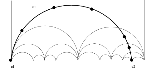
A.6.7 The Sharbly Complex for General Groups
In [Gun00b] we generalized Theorem A.22 (without
the complexity statement) to the symplectic group . Using
this algorithm and the symplectic retract [MM93, MM89], one can
compute the action of the Hecke operators on the top-degree cohomology
of subgroups of  .
.
More recently, Toth has investigated modular symbols for other groups.
He showed that the unimodular symbols generate the top-degree
cohomology groups for an arithmetic subgroup of a split
classical group or a split group of type  or
or  [Tot05]. His technique of proof is completely different from that
of [Gun00b]. In particular he does not give an analogue of the
Manin trick. Can one extract an algorithm from Toth’s proof that can
be used to explicitly compute the action of the Hecke operators on
cohomology?
[Tot05]. His technique of proof is completely different from that
of [Gun00b]. In particular he does not give an analogue of the
Manin trick. Can one extract an algorithm from Toth’s proof that can
be used to explicitly compute the action of the Hecke operators on
cohomology?
The proof of the main result of [Gun00b] uses a description of
the relations among the modular symbols. These relations were
motivated by the structure of the cell complex in [MM93, MM89].
The modular symbols and these relations are analogues of the groups
and  in the sharbly complex. Can one
extend these combinatorial constructions to form a symplectic sharbly complex?
What about for general groups ?
in the sharbly complex. Can one
extend these combinatorial constructions to form a symplectic sharbly complex?
What about for general groups ?
Already for  , resolution of this question would have immediate
arithmetic applications. Indeed, Harder has a beautiful conjecture
about certain congruences between holomorphic modular forms and Siegel
modular forms of full level [Hara]. Examples of these
congruences were checked numerically in [Hara] using techniques of
[FvdG] to compute the Hecke action.
, resolution of this question would have immediate
arithmetic applications. Indeed, Harder has a beautiful conjecture
about certain congruences between holomorphic modular forms and Siegel
modular forms of full level [Hara]. Examples of these
congruences were checked numerically in [Hara] using techniques of
[FvdG] to compute the Hecke action.
However, to investigate higher levels, one needs a different technique.
The relevant cohomology classes live in  ,
so one only needs to understand the first three terms of the complex
,
so one only needs to understand the first three terms of the complex
 . We understand ,
from [Gun00b]; the key is understanding
. We understand ,
from [Gun00b]; the key is understanding  , which
should encode relations among elements of . If one could do
this and then could generalize the techniques of [Gun00a],
one would have a way to investigate Harder’s conjecture.
, which
should encode relations among elements of . If one could do
this and then could generalize the techniques of [Gun00a],
one would have a way to investigate Harder’s conjecture.
A.6.8 Generalized Modular Symbols
We conclude this appendix by discussing a geometric approach to modular symbols. This complements the algebraic approaches presented in this book and leads to many new interesting phenomena and problems.
Suppose  and are connected semisimple algebraic groups over
with an injective map
and are connected semisimple algebraic groups over
with an injective map  . Let
. Let  be a maximal compact subgroup of
  , and suppose
  is a maximal compact subgroup containing
  . Let and
  .
.
Now let be a torsion-free arithmetic
subgroup. Let  . We get a map
 , and we
denote the image by
, and we
denote the image by  . Any
compactly supported cohomology class
. Any
compactly supported cohomology class  can be pulled back via to
  and integrated to obtain a complex number. Hence
defines a linear form on
and integrated to obtain a complex number. Hence
defines a linear form on  . By Poincar’e duality, this linear form
determines a class
. By Poincar’e duality, this linear form
determines a class ![[S (H,\Gamma )] \in H^{\dim X - \dim Y} (\Gamma
\backslash X; \C)](_images/math/4432acb7d552d6666dae499a60e14ebc3048d800.png) , called a generalized modular symbol.
Such classes have been considered by many authors,
for example
[AB90, SV03, Har05, AGR93].
, called a generalized modular symbol.
Such classes have been considered by many authors,
for example
[AB90, SV03, Har05, AGR93].
As an example, we can take to be the split form of ,
and we can take  to be the inclusion of
connected component of the diagonal subgroup. Hence
to be the inclusion of
connected component of the diagonal subgroup. Hence  . In this case is trivial. The image of in
is the ideal geodesic from to . One way to vary is by
taking an
. In this case is trivial. The image of in
is the ideal geodesic from to . One way to vary is by
taking an  -translate of this geodesic, which gives a
geodesic between two cusps. Hence we can obtain the support of any
modular symbol this way. This example generalizes to to
yield the modular symbols in Section A.4 Hecke Operators and Modular Symbols. Here
-translate of this geodesic, which gives a
geodesic between two cusps. Hence we can obtain the support of any
modular symbol this way. This example generalizes to to
yield the modular symbols in Section A.4 Hecke Operators and Modular Symbols. Here  . Note that
  , so the cohomology classes
we have constructed live in the top degree
, so the cohomology classes
we have constructed live in the top degree  .
.
Another family of examples is provided by taking to be a Levi
factor of a parabolic subgroup; these are the modular symbols studied
in [AB90].
There are many natural questions to study for such objects. Here are two:
Under what conditions on
 is
is ![[S
(H,\Gamma)]](_images/math/f1918903ad721cf7d004e496e8729fc0a7ea625f.png) nonzero? This question is connected to relations between periods
of automorphic forms and functoriality lifting. There are a variety
of partial results known; see for example [SV03, AGR93].
nonzero? This question is connected to relations between periods
of automorphic forms and functoriality lifting. There are a variety
of partial results known; see for example [SV03, AGR93].We know the usual modular symbols span the top-degree cohomology for any arithmetic group
. Fix a class of generalized modular
symbols by fixing the pair  and fixing some class of maps
. How much of the cohomology can one span for a general arithmetic
group ?
and fixing some class of maps
. How much of the cohomology can one span for a general arithmetic
group ?A simple example is given by the Ash–Borel construction for
 and a Levi factor of a rational parabolic subgroup
 of type
  . In this case
  and sits inside via
For
 these symbols define a subspace
Are there
for which  equals
the full cohomology space? For general how much is
captured? Is there
a nice combinatorial way to write down the relations among these
classes? Can one cook up a generalization of Theorem
Theorem A.22 for these classes and use it to compute Hecke
eigenvalues?
equals
the full cohomology space? For general how much is
captured? Is there
a nice combinatorial way to write down the relations among these
classes? Can one cook up a generalization of Theorem
Theorem A.22 for these classes and use it to compute Hecke
eigenvalues?
Footnotes::
| [1] | The classic references for cohomology with local systems are [Ste99a, Section 31] and [Eil47, Ch. V]. A more recent exposition (in the language of v Cech cohomology and locally constant sheaves) can be found in [BT82, II.13]. For an exposition tailored to our needs, see [Harb, Section 2.9].} |
| [2] | However, Maass forms play a very important indirect role in arithmetic. |
| [3] | The symmetric spaces that have a complex structure are known as bounded domains, or Hermitian symmetric spaces [Hel01]. |
| [4] | This apt phrase is due to Vogan [Vog97]. |
| [5] | This is a bit of an oversimplification, since it is a highly
nontrivial problem to decide when cusp cohomology from lower rank
groups appears in . However, many results are known; as a
selection we mention [Har91, Har87, LS04]. |
| [6] | Strictly speaking, Voronoi actually showed that every codimension 1 cone is contained in two top-dimensional cones. |
| [7] | If has torsion, then cells in can have
nontrivial stabilizers in , and thus
 should be considered as an “orbifold”
cellular decomposition. should be considered as an “orbifold”
cellular decomposition. |
| [8] | Under the identification
 ,
the map becomes the transfer map in group cohomology
[Bro94, III.9]. ,
the map becomes the transfer map in group cohomology
[Bro94, III.9]. |
| [9] | The first interesting case is , for which the cuspidal
cohomology lives in  . . |
| [10] | The terminology for is due to Lee Rudolph, in honor
of Lee and Szczarba. They introduced a very similar complex in
[LS76] for . |
| [11] | In fact, we can be slightly more clever than this and only
introduce denominators that are powers of . |
| [12] | Such forms are called Humbert forms in the literature. |
| [13] | Indeed, computing all simplicial subdivisions of
 is a difficult problem in convex geometry. is a difficult problem in convex geometry. |